The HPCDM Procedure(Experimental)

Scenario Analysis
The distributions of loss frequency and loss severity often depend on exogenous variables (regressors). For example, the number of losses and the severity of each loss that an automobile insurance policyholder incurs might depend on the characteristics of the policyholder and the characteristics of the vehicle. When you fit frequency and severity models, you need to account for the effects of such regressors on the probability distributions of the counts and severity. The COUNTREG procedure enables you to model regression effects on the mean of the count distribution, and the SEVERITY procedure enables you to model regression effects on the scale parameter of the severity distribution. When you use these models to estimate the compound distribution model of the aggregate loss, you need to specify a set of values for all the regressors, which represents the state of the world for which the simulation is conducted. This is referred to as the what-if or scenario analysis.
Consider that you, as an automobile insurance company, have postulated that the distribution of the loss event frequency depends on five regressors (external factors): age of the policyholder, gender, type of car, annual miles driven, and policyholder’s education level. Further, the distribution of the severity of each loss depends on three regressors: type of car, safety rating of the car, and annual household income of the policyholder (which can be thought of as a proxy for the luxury level of the car). Note that the frequency model regressors and severity model regressors can be different, as illustrated in this example.
Let these regressors be recorded in the variables Age (scaled by a factor of 1/50), Gender (1: female, 2: male), CarType (1: sedan, 2: sport utility vehicle), AnnualMiles (scaled by a factor of 1/5,000), Education (1: high school graduate, 2: college graduate, 3: advanced degree holder), CarSafety (scaled to be between 0 and 1, the safest being 1), and Income (scaled by a factor of 1/100,000), respectively. Let the historical data about the number of losses that various policyholders
incur in a year be recorded in the NumLoss variable of the Work.LossCounts data set, and let the severity of each loss be recorded in the LossAmount variable of the Work.Losses data set.
The following PROC COUNTREG step fits the count regression model and stores the fitted model information in the Work.CountregModel item store:
/* Fit negative binomial frequency model for the number of losses */
proc countreg data=losscounts;
   model numloss = age gender carType annualMiles education / dist=negbin;
   store work.countregmodel;
run;
You can examine the parameter estimates of the count model that are stored in the Work.CountregModel item store by submitting the following statements:
/* Examine the parameter estimates for the model in the item store */
proc countreg restore=work.countregmodel;
   show parameters;
run;
The "Parameter Estimates" table that is displayed by the SHOW statement is shown in Figure 18.5.
Figure 18.5: Parameter Estimates of the Count Regression Model
| Parameter Estimates | |||||
|---|---|---|---|---|---|
| Parameter | DF | Estimate | Standard Error |
t Value | Approx Pr > |t| |
| Intercept | 1 | 0.910479 | 0.090515 | 10.06 | <.0001 |
| age | 1 | -0.626803 | 0.058547 | -10.71 | <.0001 |
| gender | 1 | 1.025034 | 0.032099 | 31.93 | <.0001 |
| carType | 1 | 0.615165 | 0.031153 | 19.75 | <.0001 |
| annualMiles | 1 | -1.010276 | 0.017512 | -57.69 | <.0001 |
| education | 1 | -0.280246 | 0.021677 | -12.93 | <.0001 |
| _Alpha | 1 | 0.318403 | 0.020090 | 15.85 | <.0001 |
The following PROC SEVERITY step fits the severity scale regression models for all the common distributions that are predefined in PROC SEVERITY:
/* Fit severity models for the magnitude of losses */
proc severity data=losses plots=none outest=work.sevregest print=all;
   loss lossamount;
   scalemodel carType carSafety income;
   dist _predef_;
   nloptions maxiter=100;
run;
The comparison of fit statistics of various scale regression models is shown in Figure 18.6. The scale regression model that is based on the lognormal distribution is deemed the best-fitting model according to the likelihood-based statistics, whereas the scale regression model that is based on the generalized Pareto distribution (GPD) is deemed the best-fitting model according to the EDF-based statistics.
Figure 18.6: Severity Model Comparison
| All Fit Statistics | ||||||||||||||
|---|---|---|---|---|---|---|---|---|---|---|---|---|---|---|
| Distribution | -2 Log Likelihood |
AIC | AICC | BIC | KS | AD | CvM | |||||||
| Burr | 127231 | 127243 | 127243 | 127286 | 7.75407 | 224.47578 | 27.41346 | |||||||
| Exp | 128431 | 128439 | 128439 | 128467 | 6.13537 | 181.83094 | 12.33919 | |||||||
| Gamma | 128324 | 128334 | 128334 | 128370 | 7.54562 | 276.13156 | 24.59515 | |||||||
| Igauss | 127434 | 127444 | 127444 | 127480 | 6.15855 | 211.51908 | 17.70942 | |||||||
| Logn | 127062 | * | 127072 | * | 127072 | * | 127107 | * | 6.77687 | 212.70400 | 21.47945 | |||
| Pareto | 128166 | 128176 | 128176 | 128211 | 5.37453 | 110.53673 | 7.07119 | |||||||
| Gpd | 128166 | 128176 | 128176 | 128211 | 5.37453 | * | 110.53660 | * | 7.07116 | * | ||||
| Weibull | 128429 | 128439 | 128439 | 128475 | 6.21268 | 190.81178 | 13.45425 | |||||||
| Note: The asterisk (*) marks the best model according to each column's criterion. | ||||||||||||||
Now, you are ready to analyze the distribution of the aggregate loss that can be expected from a specific policyholder—for
example, a 59-year-old male policyholder with an advanced degree who earns 159,870 and drives a sedan that has a very high
safety rating about 11,474 miles annually. First, you need to encode and scale this information into the appropriate regressor
variables of a data set. Let that data set be named Work.SinglePolicy, with an observation as shown in Figure 18.7.
Figure 18.7: Scenario Analysis Data for One Policyholder
Now, you can submit the following PROC HPCDM step to analyze the compound distribution of the aggregate loss that is incurred
by the policyholder in the Work.SinglePolicy data set in a given year by using the frequency model from the Work.CountregModel item store and the two best severity models, lognormal and GPD, from the Work.SevRegEst data set:
/* Simulate the aggregate loss distribution for the scenario
   with single policyholder */
proc hpcdm data=singlePolicy nreplicates=10000 seed=13579 print=all
           countstore=work.countregmodel severityest=work.sevregest;
   severitymodel logn gpd;
   outsum out=onepolicysum mean stddev skew kurtosis median
         pctlpts=97.5 to 99.5 by 1;
run;
The displayed results from the preceding PROC HPCDM step are shown in Figure 18.8.
When you use a severity scale regression model, it is recommended that you verify the severity scale regressors that are used by PROC HPCDM by examining the Scale Model Regressors row of the "Compound Distribution Information" table. PROC HPCDM detects the severity regressors automatically by examining the variables in the SEVERITYEST= and DATA= data sets. If those data sets contain variables that you did not include in the SCALEMODEL statement in PROC SEVERITY, then such variables can be treated as severity regressors. One common mistake that can lead to this situation is to fit a severity model by using the BY statement and forget to specify the identical BY statement in the PROC HPCDM step; this can cause PROC HPCDM to treat BY variables as scale model regressors. In this example, Figure 18.8 confirms that the correct set of scale model regressors is detected.
Figure 18.8: Scenario Analysis Results for One Policyholder with Lognormal Severity Model
The "Sample Summary Statistics" and "Sample Percentiles" tables in Figure 18.8 show estimates of the aggregate loss distribution for the lognormal severity model. The average expected loss is about 218, and the worst-case loss, if approximated by the 97.5th percentile, is about 1,418. The percentiles table shows that the distribution is highly skewed to the right; this is also confirmed by the skewness estimate. The median estimate of 0 can be interpreted in two ways. One way is to conclude that the policyholder will not incur any loss in 50% of the years during which he or she is insured. The other way is to conclude that 50% of policyholders who have the characteristics of this policyholder will not incur any loss in a given year. However, there is a 2.5% chance that the policyholder will incur a loss that exceeds 1,418 in any given year and a 0.5% chance that the policyholder will incur a loss that exceeds 2,590 in any given year.
If the aggregate loss sample is simulated by using the GPD severity model, then the results are as shown in Figure 18.9. The average and worst-case losses are 212 and 1,388, respectively. These estimates are very close to the values that are predicted by the lognormal severity model.
Figure 18.9: Scenario Analysis Results for One Policyholder with GPD Severity Model
The scenario that you just analyzed contains only one policyholder. You can extend the scenario to include multiple policyholders.
Let the Work.GroupOfPolicies data set record information about five different policyholders, as shown in Figure 18.10.
Figure 18.10: Scenario Analysis Data for Multiple Policyholders
The following PROC HPCDM step conducts a scenario analysis for the aggregate loss that is incurred by all five policyholders
in the Work.GroupOfPolicies data set together in one year:
/* Simulate the aggregate loss distribution for the scenario
   with multiple policyholders */
proc hpcdm data=groupOfPolicies nreplicates=10000 seed=13579 print=all
           countstore=work.countregmodel severityest=work.sevregest
           plots=(conditionaldensity(rightq=0.95)) nperturbedSamples=50;
   severitymodel logn gpd;
   outsum out=multipolicysum mean stddev skew kurtosis median
         pctlpts=97.5 to 99.5 by 1;
run;
The preceding PROC HPCDM step conducts perturbation analysis by simulating 50 perturbed samples. The perturbation summary
results for the lognormal severity model are shown in Figure 18.11, and the results for the GPD severity model are shown in Figure 18.12. If the severity of each loss follows the fitted lognormal distribution, then you can expect that the group of policyholders
together incurs an average loss of 5,331  560 and a worst-case loss of 15,859 1,442 when you define the worst-case loss as the 97.5th percentile.
Figure 18.11: Perturbation Analysis of Losses from Multiple Policyholders with Lognormal Severity Model
| Sample Percentile Perturbation Analysis | ||
|---|---|---|
| Percentile | Estimate | Standard Error |
| 1 | 216.43966 | 65.57200 |
| 5 | 765.60278 | 143.70919 |
| 25 | 2401.0 | 324.11066 |
| 50 | 4342.7 | 498.47507 |
| 75 | 7139.4 | 739.01751 |
| 95 | 13185.9 | 1217.8 |
| 97.5 | 15858.5 | 1441.8 |
| 98.5 | 17886.4 | 1585.0 |
| 99 | 19553.1 | 1693.9 |
| 99.5 | 22646.0 | 2001.5 |
| Number of Perturbed Samples = 50 | ||
| Size of Each Sample = 10000 | ||
If the severity of each loss follows the fitted GPD distribution, then you can expect an average loss of 5,294 539 and a worst-case loss of 15,128 1,340.
If you decide to use the 99.5th percentile to define the worst-case loss, then the worst-case loss is 22,646 2,002 for the lognormal severity model and 20,539 1,798 for the GPD severity model. The numbers for lognormal and GPD are well within one standard error of each other, which
indicates that the aggregate loss distribution is less sensitive to the choice of these two severity distributions in this
particular example; you can use the results from either of them.
Figure 18.12: Perturbation Analysis of Losses from Multiple Policyholders with GPD Severity Model
| Sample Percentile Perturbation Analysis | ||
|---|---|---|
| Percentile | Estimate | Standard Error |
| 1 | 173.75335 | 62.52659 |
| 5 | 728.89376 | 137.91935 |
| 25 | 2422.1 | 314.53125 |
| 50 | 4424.5 | 488.71163 |
| 75 | 7204.9 | 710.03240 |
| 95 | 12851.4 | 1180.1 |
| 97.5 | 15127.8 | 1340.4 |
| 98.5 | 16823.9 | 1482.5 |
| 99 | 18206.7 | 1621.8 |
| 99.5 | 20538.9 | 1797.6 |
| Number of Perturbed Samples = 50 | ||
| Size of Each Sample = 10000 | ||
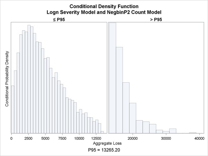
The PLOTS=CONDITIONALDENSITY option that is used in the preceding PROC HPCDM step prepares the conditional density plots for
the body and right-tail regions of the density function of the aggregate loss. The plots for the aggregate loss sample that
is generated by using the lognormal severity model are shown in Figure 18.13. The plot on the left side is the plot of  , where the limit 13,265 is the 95th percentile as specified by the RIGHTQ=0.95 option. The plot on the right side is the
plot of
, where the limit 13,265 is the 95th percentile as specified by the RIGHTQ=0.95 option. The plot on the right side is the
plot of  , which helps you visualize the right-tail region of the density function. You can also request the plot of the left tail
by specifying the LEFTQ= suboption of the CONDITIONALDENSITY option if you want to explore the details of the left tail region.
Note that the conditional density plots are always produced by using the unperturbed sample.
, which helps you visualize the right-tail region of the density function. You can also request the plot of the left tail
by specifying the LEFTQ= suboption of the CONDITIONALDENSITY option if you want to explore the details of the left tail region.
Note that the conditional density plots are always produced by using the unperturbed sample.
Figure 18.13: Conditional Density Plots for the Aggregate Loss of Multiple Policyholders