The HPCDM Procedure(Experimental)

This example illustrates the simplest use of PROC HPCDM. Assume that you are an insurance company that has used the historical data about the number of losses per year and the severity of each loss to determine that the Poisson distribution is the best distribution for the loss frequency and that the gamma distribution is the best distribution for the severity of each loss. Now, you want to estimate the distribution of an aggregate loss to determine the worst-case loss that can be incurred by your policyholders in a year. In other words, you want to estimate the compound distribution of , where the loss frequency, N, follows the fitted Poisson distribution and the severity of each loss event, , follows the fitted gamma distribution.

If your historical count and severity data are stored in the data sets Work.ClaimCount and Work.ClaimSev, respectively, then you need to ensure that you use the following PROC COUNTREG and PROC SEVERITY steps to fit and store the parameter estimates of the frequency and severity models:

/* Fit an intercept-only Poisson count model and
   write estimates to an item store */
proc countreg data=claimcount;
   model numLosses= / dist=poisson;
   store countStorePoisson;
run;

/* Fit severity models and write estimates to a data set */
proc severity data=claimsev criterion=aicc outest=sevest covout plots=none;
   loss lossValue;
   dist _predefined_;
run;

The STORE statement in the PROC COUNTREG step saves the count model information, including the parameter estimates, in the Work.CountStorePoisson item store. An item store contains the model information in a binary format that cannot be modified after it is created. You can examine the contents of an item store that is created by a PROC COUNTREG step by specifying a combination of the RESTORE= option and the SHOW statement in another PROC COUNTREG step. For more information, see Chapter 12: The COUNTREG Procedure.

The OUTEST= option in the PROC SEVERITY statement stores the estimates of all the fitted severity models in the Work.SevEst data set. Let the best severity model that the PROC SEVERITY step chooses be the gamma distribution model.

You can now submit the following PROC HPCDM step to simulate an aggregate loss sample of size 10,000 by specifying the count model’s item store in the COUNTSTORE= option and the severity model’s data set of estimates in the SEVERITYEST= option:

/* Simulate and estimate Poisson-gamma compound distribution model */
proc hpcdm countstore=countStorePoisson severityest=sevest
           seed=13579 nreplicates=10000 plots=(edf(alpha=0.05) density)
           print=(summarystatistics percentiles);
   severitymodel gamma;
   output out=aggregateLossSample samplevar=aggloss;
   outsum out=aggregateLossSummary mean stddev skewness kurtosis
          p01 p05 p95 p995=var pctlpts=90 97.5;
run;

The SEVERITYMODEL statement requests that an aggregate sample be generated by compounding only the gamma distribution and the frequency distribution. Specifying the SEED= value helps you get an identical sample each time you execute this step, provided that you use the same execution environment. In the single-machine mode of execution, the execution environment is the combination of the operating environment and the number of threads that are used for execution. In the distributed computing mode, the execution environment is the combination of the operating environment, the number of nodes, and the number of threads that are used for execution on each node.

Upon completion, PROC HPCDM creates the two output data sets that you specify in the OUT= options of the OUTPUT and OUTSUM statements. The Work.AggregateLossSample data set contains 10,000 observations such that the value of the AggLoss variable in each observation represents one possible aggregate loss value that you can expect to see in one year. Together, the set of the 10,000 values of the AggLoss variable represents one sample of compound distribution. PROC HPCDM uses this sample to compute the empirical estimates of various summary statistics and percentiles of the compound distribution. The Work.AggregateLossSummary data set contains the estimates of mean, standard deviation, skewness, and kurtosis that you specify in the OUTSUM statement. It also contains the estimates of the 1st, 5th, 90th, 95th, 97.5th, and 99.5th percentiles that you specify in the OUTSUM statement. The value-at-risk (VaR) is an aggregate loss value such that there is a very low probability that an observed aggregate loss value exceeds the VaR. One of the commonly used probability levels to define VaR is 0.005, which makes the 99.5th percentile an empirical estimate of the VaR. Hence, the OUTSUM statement of this example stores the 99.5th percentile in a variable named VaR. VaR is one of the widely used measures of worst-case risk.

Some of the default output and some of the output that you have requested by specifying the PRINT= option are shown in Figure 18.1.

The "Sample Summary Statistics" table indicates that for the given parameter estimates of the Poisson frequency and gamma severity models, you can expect to see a mean aggregate loss of 4,062.8 and a median aggregate loss of 3,349.7 in a year. The "Sample Percentiles" table indicates that there is a 0.5% chance that the aggregate loss exceeds 15,877.9, which is the VaR estimate, and a 2.5% chance that the aggregate loss exceeds 12,391.7. These summary statistic and percentile estimates provide a quantitative picture of the compound distribution. You can also visually analyze the compound distribution by examining the plots that PROC HPCDM prepares. The first plot in Figure 18.2 shows the empirical distribution function (EDF), which is a nonparametric estimate of the cumulative distribution function (CDF). The second plot shows the histogram and the kernel density estimate, which are nonparametric estimates of the probability density function (PDF).

Figure 18.2: Nonparametric CDF and PDF Plots of the Poisson-Gamma Compound Distribution

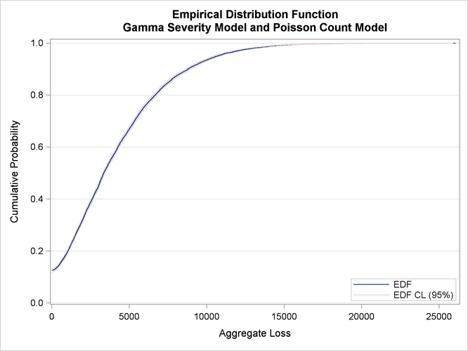
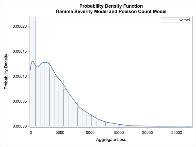
The plots confirm the right skew that is indicated by the estimate of skewness in Figure 18.1 and a relatively fat tail, which is indicated by comparing the maximum and the 99.5th percentiles in Figure 18.1.