The FORECAST Procedure
- Overview
-
Getting Started
 Giving Dates to Forecast ValuesComputing Confidence LimitsForm of the OUT= Data SetPlotting ForecastsPlotting ResidualsModel Parameters and Goodness-of-Fit StatisticsControlling the Forecasting MethodIntroduction to Forecasting MethodsTime Trend ModelsTime Series MethodsCombining Time Trend with Autoregressive Models
 -
Syntax
-
Details
-
Examples
- References
Time Series Methods
Time series models assume the future value of a variable to be a linear function of past values. If the model is a function of past values for a finite number of periods, it is an autoregressive model and is written as follows:
![\[ x_{t}=a_{0}+a_{1}x_{t-1} +a_{2}x_{t-2}+\ldots +a_{p}x_{t-p}+{\epsilon }_{t} \]](images/etsug_forecast0010.png)
The coefficients a are autoregressive parameters. One of the simplest cases of this model is the random walk, where the series dances around in purely random jumps. This
is illustrated in Figure 17.10.
are autoregressive parameters. One of the simplest cases of this model is the random walk, where the series dances around in purely random jumps. This
is illustrated in Figure 17.10.
Figure 17.10: Random Walk Series
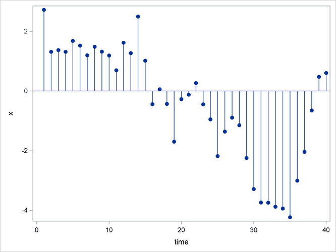
The  values are generated by the equation
![\[ x_{t}=x_{t-1}+{\epsilon }_{t} \]](images/etsug_forecast0013.png)
In this type of model, the best forecast of a future value is the present value. However, with other autoregressive models, the best forecast is a weighted sum of recent values. Pure autoregressive forecasts always damp down to a constant (assuming the process is stationary).
Autoregressive time series models can also be used to predict seasonal fluctuations.