The COPULA Procedure
- Overview
- Getting Started
-
Syntax

-
DetailsSklar’s TheoremDependence MeasuresNormal CopulaStudent’s t copulaArchimedean CopulasHierarchical Archimedean Copula (HAC)Canonical Maximum Likelihood Estimation (CMLE)Exact Maximum Likelihood Estimation (MLE)Calibration EstimationNonlinear Optimization OptionsDisplayed OutputOUTCOPULA= Data SetOUTPSEUDO=, OUT=, and OUTUNIFORM= Data SetsODS Table NamesODS Graph Names
-
Examples
- References
Getting Started: COPULA Procedure
The following example illustrates the use of PROC COPULA. The data used are daily returns on several major stocks. The main purpose of this example is to estimate the joint distribution of stock returns and then simulate from this distribution a new sample of specified size.
Figure 11.1 shows the first 10 observations of the daily stock return data set.
Figure 11.1: First 10 Observations of Daily Returns
| Obs | date | ret_msft | ret_ko | ret_ibm | ret_duk | ret_bp |
|---|---|---|---|---|---|---|
| 1 | 01/03/2008 | 0.004182 | 0.010367 | 0.002002 | 0.003503 | 0.019114 |
| 2 | 01/04/2008 | -0.027960 | 0.001913 | -0.035861 | -0.000582 | -0.014536 |
| 3 | 01/07/2008 | 0.006732 | 0.023607 | -0.010671 | 0.025611 | 0.017922 |
| 4 | 01/08/2008 | -0.033435 | 0.004239 | -0.024610 | -0.002838 | -0.016049 |
| 5 | 01/09/2008 | 0.029560 | 0.026680 | 0.007301 | 0.010814 | -0.027078 |
| 6 | 01/10/2008 | -0.003054 | 0.004441 | 0.016414 | -0.001689 | -0.004395 |
| 7 | 01/11/2008 | -0.012255 | -0.027346 | -0.022546 | -0.012408 | -0.018473 |
| 8 | 01/14/2008 | 0.013958 | 0.008418 | 0.053857 | 0.003427 | 0.001166 |
| 9 | 01/15/2008 | -0.011318 | -0.010851 | -0.010689 | -0.017075 | -0.040925 |
| 10 | 01/16/2008 | -0.022587 | -0.015021 | -0.001955 | 0.002316 | -0.021336 |
The following statements fit a normal copula to the returns data (with the FIT statement) and create a new SAS data set that contains parameter estimates of the model. The VAR statement specifies the list of variables, which in this case are the daily returns of five large company stocks.
/* Copula estimation */
proc copula data = returns;
   var ret_ibm ret_msft ret_bp ret_ko ret_duk;
   fit normal / outcopula=estimates;
run;
The first table in Figure 11.2 shows some general information about the copula fitting procedure: the number of observations, the name of the input data set, the type of model and the correlation matrix.
Figure 11.2: Copula Estimation: Fit Summary and Correlation Matrix
Next, the following statements restrict the data set to only those columns that contain correlation parameter estimates.
/* keep only correlation estimates */
data estimates;
   set estimates;
   keep ret_ibm ret_msft ret_bp ret_ko ret_duk;
run;
Then, in the following statements, the DEFINE statement specifies a normal copula named COP, and the CORR= option specifies
that the data set Estimates be used as the source for the model parameters. The NDRAWS=500 option in the SIMULATE statement generates 500 observations
from the normal copula. The OUTUNIFORM= option specifies the name of SAS data set to contain the simulated sample with uniform
marginal distributions. Note that this syntax does not require the DATA= option.
/* Copula simulation of uniforms */
proc copula;
   var ret_ibm ret_msft ret_bp ret_ko ret_duk;
   define cop normal (corr = estimates);
   simulate cop / ndraws     = 500
                  seed       = 1234
                  outuniform = simulated_uniforms
                  plots=(datatype=uniform);
run;
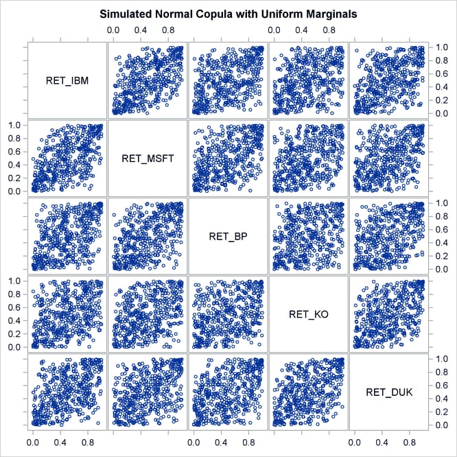
The simulated data is contained in the new SAS data set, Simulated_Uniforms. A scatter plot matrix of uniform marginals contained in the data set is shown in Figure 11.3.
Figure 11.3: Simulated Data, Uniform Marginals
The preceding sequence of PROC COPULA usage—first fit, then simulate given estimated parameters—is a legitimate sequence but has a limitation in that the second COPULA call does not generate the sample according to the empirical distribution of the raw data. It generates only marginally uniform series.
In the following statements, the FIT statement fits a t copula to the returns data and at the same time simulates the sample according to empirical marginal distributions:
/* Copula estimation and simulation of returns */
proc copula data = returns;
   var ret_ibm ret_msft ret_bp ret_ko ret_duk;
   fit T;
   simulate / ndraws = 1000
              seed   = 1234
              out    = simulated_returns;
run;
The output of the statements is similar in structure to the output displayed in Figure 11.2 with the addition of parameter estimates and inference statistics that are specific to the copula model as shown in Figure 11.4. For a t copula, the degrees of freedom are displayed (as in Figure 11.4); for Archimedean copulas, the parameter "theta" is displayed; and for a normal copula, this table is not printed.
Figure 11.4: Copula Estimation: Specific Parameter Estimates
The simulated data is contained in the new SAS data set, Simulated_Returns.