The ARIMA Procedure
- Overview
-
Getting Started
 The Three Stages of ARIMA ModelingIdentification StageEstimation and Diagnostic Checking StageForecasting StageUsing ARIMA Procedure StatementsGeneral Notation for ARIMA ModelsStationarityDifferencingSubset, Seasonal, and Factored ARMA ModelsInput Variables and Regression with ARMA ErrorsIntervention Models and Interrupted Time SeriesRational Transfer Functions and Distributed Lag ModelsForecasting with Input VariablesData Requirements
 -
Syntax
-
DetailsThe Inverse Autocorrelation FunctionThe Partial Autocorrelation FunctionThe Cross-Correlation FunctionThe ESACF MethodThe MINIC MethodThe SCAN MethodStationarity TestsPrewhiteningIdentifying Transfer Function ModelsMissing Values and AutocorrelationsEstimation DetailsSpecifying Inputs and Transfer FunctionsInitial ValuesStationarity and InvertibilityNaming of Model ParametersMissing Values and Estimation and ForecastingForecasting DetailsForecasting Log Transformed DataSpecifying Series PeriodicityDetecting OutliersOUT= Data SetOUTCOV= Data SetOUTEST= Data SetOUTMODEL= SAS Data SetOUTSTAT= Data SetPrinted OutputODS Table NamesStatistical Graphics
-
Examples
- References
Identification Stage
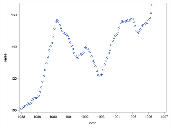
Suppose you have a variable called SALES that you want to forecast. The following example illustrates ARIMA modeling and forecasting by using a simulated data set
TEST that contains a time series SALES generated by an ARIMA(1,1,1) model. The output produced by this example is explained in the following sections. The simulated
SALES series is shown in Figure 8.1.
proc sgplot data=test;
   scatter y=sales x=date;
run;
Figure 8.1: Simulated ARIMA(1,1,1) Series SALES
Using the IDENTIFY Statement
You first specify the input data set in the PROC ARIMA statement. Then, you use an IDENTIFY statement to read in the SALES series and analyze its correlation properties. You do this by using the following statements:
proc arima data=test ;
   identify var=sales nlag=24;
run;
Descriptive Statistics
The IDENTIFY statement first prints descriptive statistics for the SALES series. This part of the IDENTIFY statement output is shown in Figure 8.2.
Figure 8.2: IDENTIFY Statement Descriptive Statistics Output
Autocorrelation Function Plots
The IDENTIFY statement next produces a panel of plots used for its autocorrelation and trend analysis. The panel contains the following plots:
-
the time series plot of the series
-
the sample autocorrelation function plot (ACF)
-
the sample inverse autocorrelation function plot (IACF)
-
the sample partial autocorrelation function plot (PACF)
This correlation analysis panel is shown in Figure 8.3.
Figure 8.3: Correlation Analysis of SALES
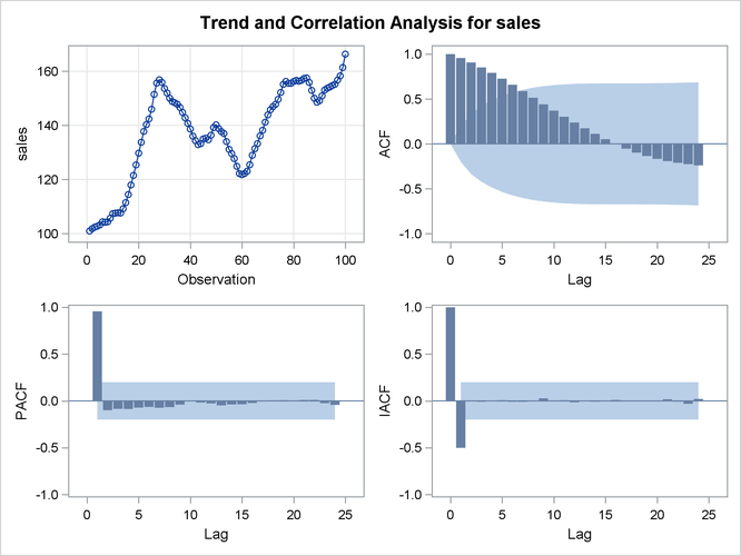
These autocorrelation function plots show the degree of correlation with past values of the series as a function of the number of periods in the past (that is, the lag) at which the correlation is computed.
The NLAG= option controls the number of lags for which the autocorrelations are shown. By default, the autocorrelation functions are plotted to lag 24.
Most books on time series analysis explain how to interpret the autocorrelation and the partial autocorrelation plots. See the section The Inverse Autocorrelation Function for a discussion of the inverse autocorrelation plots.
By examining these plots, you can judge whether the series is stationary or nonstationary.
In this case, a visual inspection of the autocorrelation function plot indicates that the SALES series is nonstationary, since the ACF decays very slowly. For more formal stationarity tests, use the STATIONARITY= option.
(See the section Stationarity.)
White Noise Test
The last part of the default IDENTIFY statement output is the check for white noise. This is an approximate statistical test of the hypothesis that none of the autocorrelations of the series up to a given lag are significantly different from 0. If this is true for all lags, then there is no information in the series to model, and no ARIMA model is needed for the series.
The autocorrelations are checked in groups of six, and the number of lags checked depends on the NLAG= option. The check for white noise output is shown in Figure 8.4.
Figure 8.4: IDENTIFY Statement Check for White Noise
| Autocorrelation Check for White Noise | |||||||||
|---|---|---|---|---|---|---|---|---|---|
| To Lag | Chi-Square | DF | Pr > ChiSq | Autocorrelations | |||||
| 6 | 426.44 | 6 | <.0001 | 0.957 | 0.907 | 0.852 | 0.791 | 0.726 | 0.659 |
| 12 | 547.82 | 12 | <.0001 | 0.588 | 0.514 | 0.440 | 0.370 | 0.303 | 0.238 |
| 18 | 554.70 | 18 | <.0001 | 0.174 | 0.112 | 0.052 | -0.004 | -0.054 | -0.098 |
| 24 | 585.73 | 24 | <.0001 | -0.135 | -0.167 | -0.192 | -0.211 | -0.227 | -0.240 |
In this case, the white noise hypothesis is rejected very strongly, which is expected since the series is nonstationary. The p-value for the test of the first six autocorrelations is printed as <0.0001, which means the p-value is less than 0.0001.
Identification of the Differenced Series
Since the series is nonstationary, the next step is to transform it to a stationary series by differencing. That is, instead
of modeling the SALES series itself, you model the change in SALES from one period to the next. To difference the SALES series, use another IDENTIFY statement and specify that the first difference of SALES be analyzed, as shown in the following statements:
proc arima data=test;
   identify var=sales(1);
run;
The second IDENTIFY statement produces the same information as the first, but for the change in SALES from one period to the next rather than for the total SALES in each period. The summary statistics output from this IDENTIFY statement is shown in Figure 8.5. Note that the period of differencing is given as 1, and one observation was lost through the differencing operation.
Figure 8.5: IDENTIFY Statement Output for Differenced Series
The autocorrelation plots for the differenced series are shown in Figure 8.6.
Figure 8.6: Correlation Analysis of the Change in SALES
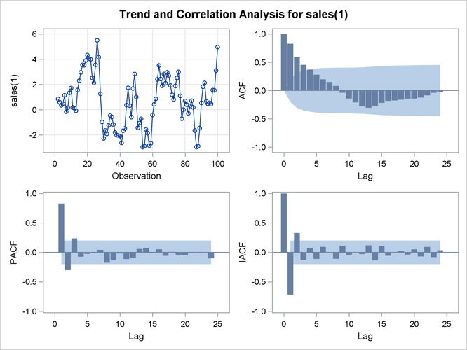
The autocorrelations decrease rapidly in this plot, indicating that the change in SALES is a stationary time series.
The next step in the Box-Jenkins methodology is to examine the patterns in the autocorrelation plot to choose candidate ARMA models to the series. The partial and inverse autocorrelation function plots are also useful aids in identifying appropriate ARMA models for the series.
In the usual Box-Jenkins approach to ARIMA modeling, the sample autocorrelation function, inverse autocorrelation function, and partial autocorrelation function are compared with the theoretical correlation functions expected from different kinds of ARMA models. This matching of theoretical autocorrelation functions of different ARMA models to the sample autocorrelation functions computed from the response series is the heart of the identification stage of Box-Jenkins modeling. Most textbooks on time series analysis, such as Pankratz (1983), discuss the theoretical autocorrelation functions for different kinds of ARMA models.
Since the input data are only a limited sample of the series, the sample autocorrelation functions computed from the input
series only approximate the true autocorrelation function of the process that generates the series. This means that the sample
autocorrelation functions do not exactly match the theoretical autocorrelation functions for any ARMA model and can have a
pattern similar to that of several different ARMA models. If the series is white noise (a purely random process), then there
is no need to fit a model. The check for white noise, shown in Figure 8.7, indicates that the change in SALES is highly autocorrelated. Thus, an autocorrelation model, for example an AR(1) model, might be a good candidate model to
fit to this process.
Figure 8.7: IDENTIFY Statement Check for White Noise
| Autocorrelation Check for White Noise | |||||||||
|---|---|---|---|---|---|---|---|---|---|
| To Lag | Chi-Square | DF | Pr > ChiSq | Autocorrelations | |||||
| 6 | 154.44 | 6 | <.0001 | 0.828 | 0.591 | 0.454 | 0.369 | 0.281 | 0.198 |
| 12 | 173.66 | 12 | <.0001 | 0.151 | 0.081 | -0.039 | -0.141 | -0.210 | -0.274 |
| 18 | 209.64 | 18 | <.0001 | -0.305 | -0.271 | -0.218 | -0.183 | -0.174 | -0.161 |
| 24 | 218.04 | 24 | <.0001 | -0.144 | -0.141 | -0.125 | -0.085 | -0.040 | -0.032 |