The ARIMA Procedure

Example 8.2 Seasonal Model for the Airline Series

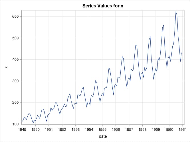
The airline passenger data, given as Series G in Box and Jenkins (1976), have been used in time series analysis literature as an example of a nonstationary seasonal time series. This example uses PROC ARIMA to fit the airline model, ARIMA(0,1,1) ${\times }$ (0,1,1) $_{12}$ , to Box and Jenkins’ Series G. The following statements read the data and log-transform the series:

title1 'International Airline Passengers';
title2 '(Box and Jenkins Series-G)';
data seriesg;
   input x @@;
   xlog = log( x );
   date = intnx( 'month', '31dec1948'd, _n_ );
   format date monyy.;
datalines;
112 118 132 129 121 135 148 148 136 119 104 118

   ... more lines ...

The following PROC TIMESERIES step plots the series, as shown in Output 8.2.1:

proc timeseries data=seriesg plot=series;
   id date interval=month;
   var x;
run;

Output 8.2.1: Time Series Plot of the Airline Passenger Series

The following statements specify an ARIMA(0,1,1) ${\times }$ (0,1,1) $_{12}$ model without a mean term to the logarithms of the airline passengers series, xlog. The model is forecast, and the results are stored in the data set B.

/*-- Seasonal Model for the Airline Series --*/
proc arima data=seriesg;
   identify var=xlog(1,12);
   estimate q=(1)(12) noint method=ml;
   forecast id=date interval=month printall out=b;
run;

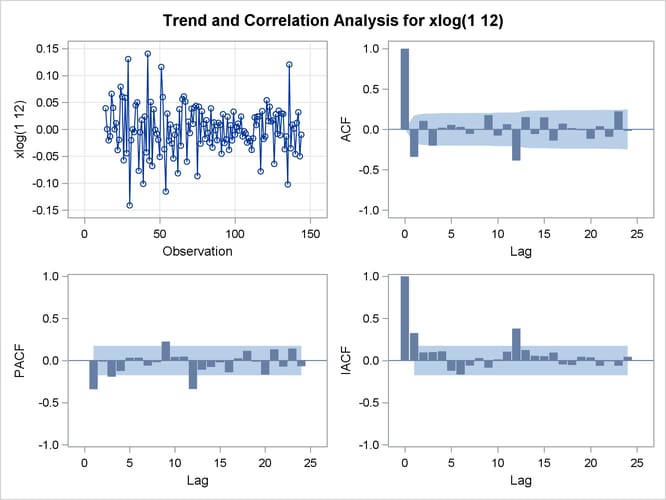
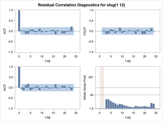
The output from the IDENTIFY statement is shown in Output 8.2.2. The autocorrelation plots shown are for the twice differenced series ${(1-{B})(1-{B}^{12})XLOG}$ . Note that the autocorrelation functions have the pattern characteristic of a first-order moving-average process combined with a seasonal moving-average process with lag 12.

Output 8.2.2: IDENTIFY Statement Output

International Airline Passengers

(Box and Jenkins Series-G)

The ARIMA Procedure

Name of Variable = xlog
Period(s) of Differencing	1,12
Mean of Working Series	0.000291
Standard Deviation	0.045673
Number of Observations	131
Observation(s) eliminated by differencing	13

Output 8.2.3: Trend and Correlation Analysis for the Twice Differenced Series

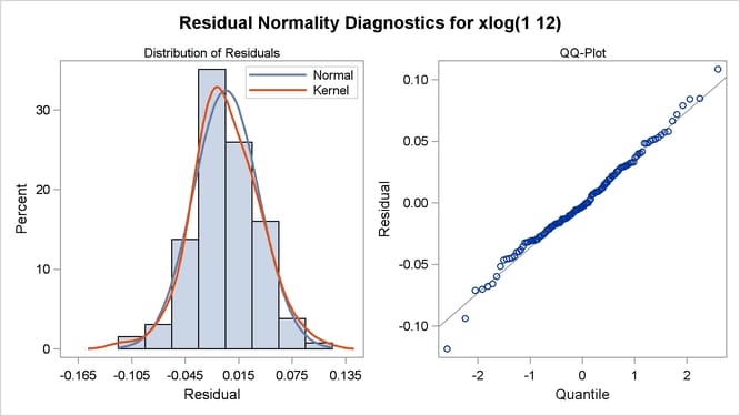
The results of the ESTIMATE statement are shown in Output 8.2.4, Output 8.2.5, and Output 8.2.6. The model appears to fit the data quite well.

Output 8.2.4: ESTIMATE Statement Output

Maximum Likelihood Estimation
Parameter	Estimate	Standard Error	t Value	Approx Pr > \|t\|	Lag
MA1,1	0.40194	0.07988	5.03	<.0001	1
MA2,1	0.55686	0.08403	6.63	<.0001	12

Variance Estimate	0.001369
Std Error Estimate	0.037
AIC	-485.393
SBC	-479.643
Number of Residuals	131

Model for variable xlog
Period(s) of Differencing	1,12

Moving Average Factors
Factor 1:	1 - 0.40194 B**(1)
Factor 2:	1 - 0.55686 B**(12)

Output 8.2.5: Residual Analysis of the Airline Model: Correlation

Output 8.2.6: Residual Analysis of the Airline Model: Normality

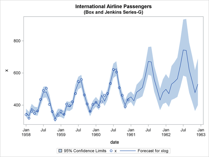
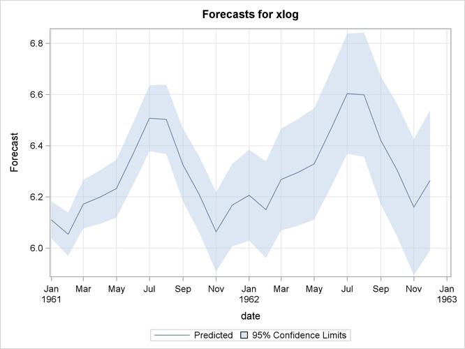
The forecasts and their confidence limits for the transformed series are shown in Output 8.2.7.

Output 8.2.7: Forecast Plot for the Transformed Series

The following statements retransform the forecast values to get forecasts in the original scales. See the section Forecasting Log Transformed Data for more information.

data c;
   set b;
   x        = exp( xlog );
   forecast = exp( forecast + std*std/2 );
   l95      = exp( l95 );
   u95      = exp( u95 );
run;

The forecasts and their confidence limits are plotted by using the following PROC SGPLOT step. The plot is shown in Output 8.2.8.

proc sgplot data=c;
   where date >= '1jan58'd;
   band Upper=u95 Lower=l95 x=date
      / LegendLabel="95% Confidence Limits";
   scatter x=date y=x;
   series x=date y=forecast;
run;

Output 8.2.8: Plot of the Forecast for the Original Series