The UCM Procedure
- Overview
-
Getting Started

-
SyntaxFunctional SummaryPROC UCM StatementAUTOREG StatementBLOCKSEASON StatementBY StatementCYCLE StatementDEPLAG StatementESTIMATE StatementFORECAST StatementID StatementIRREGULAR StatementLEVEL StatementMODEL StatementNLOPTIONS StatementOUTLIER StatementPERFORMANCE StatementRANDOMREG StatementSEASON StatementSLOPE StatementSPLINEREG StatementSPLINESEASON Statement
-
Details
-
Examples
- References
The airline passenger series, given as Series G in Box and Jenkins (1976), is often used in time series literature as an example of a nonstationary seasonal time series. This series is a monthly
series consisting of the number of airline passengers who traveled during the years 1949 to 1960. Its main features are a
steady rise in the number of passengers from year to year and the seasonal variation in the numbers during any given year.
It also exhibits an increase in variability around the trend. A ![]() transformation is used to stabilize this variability. The following DATA step prepares the
transformation is used to stabilize this variability. The following DATA step prepares the ![]() -transformed passenger series analyzed in this example:
-transformed passenger series analyzed in this example:
data seriesG;
   set sashelp.air;
   logair = log( air );
run;
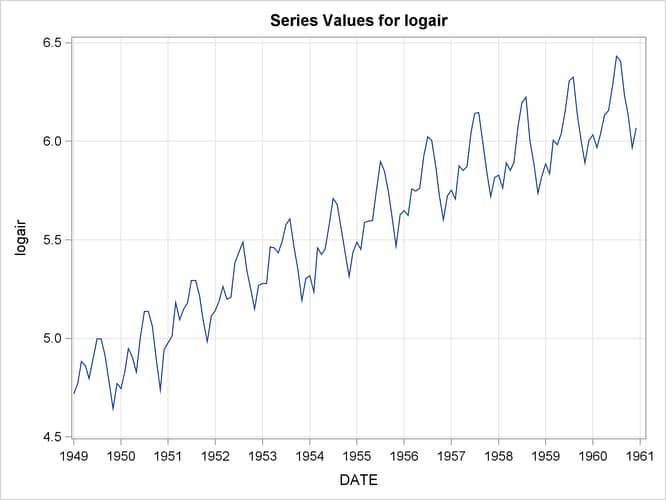
The following statements produce a time series plot of the series by using the TIMESERIES procedure (see Chapter 32: The TIMESERIES Procedure). The trend and seasonal features of the series are apparent in the plot in Figure 34.1.
proc timeseries data=seriesG plot=series;
   id date interval=month;
   var logair;
run;
In this example this series is modeled using an unobserved component model called the basic structural model (BSM). The BSM
models a time series as a sum of three stochastic components: a trend component ![]() , a seasonal component
, a seasonal component ![]() , and random error
, and random error ![]() . Formally, a BSM for a response series
. Formally, a BSM for a response series ![]() can be described as
can be described as
Each of the stochastic components in the model is modeled separately. The random error ![]() , also called the irregular component, is modeled simply as a sequence of independent, identically distributed (i.i.d.) zero-mean Gaussian random variables. The
trend and the seasonal components can be modeled in a few different ways. The model for trend used here is called a locally linear time trend. This trend model can be written as follows:
, also called the irregular component, is modeled simply as a sequence of independent, identically distributed (i.i.d.) zero-mean Gaussian random variables. The
trend and the seasonal components can be modeled in a few different ways. The model for trend used here is called a locally linear time trend. This trend model can be written as follows:
These equations specify a trend where the level ![]() as well as the slope
as well as the slope ![]() is allowed to vary over time. This variation in slope and level is governed by the variances of the disturbance terms
is allowed to vary over time. This variation in slope and level is governed by the variances of the disturbance terms ![]() and
and ![]() in their respective equations. Some interesting special cases of this model arise when you manipulate these disturbance variances.
For example, if the variance of
in their respective equations. Some interesting special cases of this model arise when you manipulate these disturbance variances.
For example, if the variance of ![]() is zero, the slope will be constant (equal to
is zero, the slope will be constant (equal to ![]() ); if the variance of
); if the variance of ![]() is also zero,
is also zero, ![]() will be a deterministic trend given by the line
will be a deterministic trend given by the line ![]() . The seasonal model used in this example is called a trigonometric seasonal. The stochastic equations governing a trigonometric
seasonal are explained later (see the section Modeling Seasons). However, it is interesting to note here that this seasonal model reduces to the familiar regression with deterministic
seasonal dummies if the variance of the disturbance terms in its equations is equal to zero. The following statements specify
a BSM with these three components:
. The seasonal model used in this example is called a trigonometric seasonal. The stochastic equations governing a trigonometric
seasonal are explained later (see the section Modeling Seasons). However, it is interesting to note here that this seasonal model reduces to the familiar regression with deterministic
seasonal dummies if the variance of the disturbance terms in its equations is equal to zero. The following statements specify
a BSM with these three components:
proc ucm data=seriesG;
   id date interval=month;
   model logair;
   irregular;
   level;
   slope;
   season length=12 type=trig print=smooth;
   estimate;
   forecast lead=24 print=decomp;
run;
The PROC UCM statement signifies the start of the UCM procedure, and the input data set, seriesG, containing the dependent series is specified there. The optional ID statement is used to specify a date, datetime, or time identification variable, date in this example, to label the observations. The INTERVAL=MONTH option in the ID statement indicates that the measurements
were collected on a monthly basis. The model specification begins with the MODEL statement, where the response series is specified (logair in this case). After this the components in the model are specified using separate statements that enable you to control
their individual properties. The irregular component ![]() is specified using the IRREGULAR statement and the trend component
is specified using the IRREGULAR statement and the trend component ![]() is specified using the LEVEL and SLOPE statements. The seasonal component
is specified using the LEVEL and SLOPE statements. The seasonal component ![]() is specified using the SEASON statement. The specifics of the seasonal characteristics such as the season length, its stochastic evolution properties,
etc., are specified using the options in the SEASON statement. The seasonal component used in this example has a season length
of 12, corresponding to the monthly seasonality, and is of the trigonometric type. Different types of seasonals are explained later (see the section Modeling Seasons).
is specified using the SEASON statement. The specifics of the seasonal characteristics such as the season length, its stochastic evolution properties,
etc., are specified using the options in the SEASON statement. The seasonal component used in this example has a season length
of 12, corresponding to the monthly seasonality, and is of the trigonometric type. Different types of seasonals are explained later (see the section Modeling Seasons).
The parameters of this model are the variances of the disturbance terms in the evolution equations of ![]() ,
, ![]() , and
, and ![]() and the variance of the irregular component
and the variance of the irregular component ![]() . These parameters are estimated by maximizing the likelihood of the data. The ESTIMATE statement options can be used to specify the span of data used in parameter estimation and to display and save the results
of the estimation step and the model diagnostics. You can use the estimated model to obtain the forecasts of the series as
well as the components. The options in the individual component statements can be used to display the component forecasts—for
example, PRINT=SMOOTH option in the SEASON statement requests the displaying of smoothed forecasts of the seasonal component
. These parameters are estimated by maximizing the likelihood of the data. The ESTIMATE statement options can be used to specify the span of data used in parameter estimation and to display and save the results
of the estimation step and the model diagnostics. You can use the estimated model to obtain the forecasts of the series as
well as the components. The options in the individual component statements can be used to display the component forecasts—for
example, PRINT=SMOOTH option in the SEASON statement requests the displaying of smoothed forecasts of the seasonal component
![]() . The series forecasts and forecasts of the sum of components can be requested using the FORECAST statement. The option PRINT=DECOMP in the FORECAST statement requests the printing of the smoothed trend
. The series forecasts and forecasts of the sum of components can be requested using the FORECAST statement. The option PRINT=DECOMP in the FORECAST statement requests the printing of the smoothed trend ![]() and the trend plus seasonal component (
and the trend plus seasonal component (![]() ).
).
The parameter estimates for this model are displayed in Figure 34.2.
Figure 34.2: BSM for the Logair Series
| Final Estimates of the Free Parameters | |||||
|---|---|---|---|---|---|
| Component | Parameter | Estimate | Approx Std Error |
t Value | Approx Pr > |t| |
| Irregular | Error Variance | 0.00023436 | 0.0001079 | 2.17 | 0.0298 |
| Level | Error Variance | 0.00029828 | 0.0001057 | 2.82 | 0.0048 |
| Slope | Error Variance | 8.47916E-13 | 6.2271E-10 | 0.00 | 0.9989 |
| Season | Error Variance | 0.00000356 | 1.32347E-6 | 2.69 | 0.0072 |
The estimates suggest that except for the slope component, the disturbance variances of all the components are significant—that
is, all these components are stochastic. The slope component, however, appears to be deterministic because its error variance is quite insignificant. It might then
be useful to check if the slope component can be dropped from the model—that is, if ![]() . This can be checked by examining the significance analysis table of the components given in Figure 34.3.
. This can be checked by examining the significance analysis table of the components given in Figure 34.3.
Figure 34.3: Component Significance Analysis for the Logair Series
| Significance Analysis of Components (Based on the Final State) |
|||
|---|---|---|---|
| Component | DF | Chi-Square | Pr > ChiSq |
| Irregular | 1 | 0.08 | 0.7747 |
| Level | 1 | 117867 | <.0001 |
| Slope | 1 | 43.78 | <.0001 |
| Season | 11 | 507.75 | <.0001 |
This table provides the significance of the components in the model at the end of the estimation span. If a component is deterministic, this analysis is equivalent to checking whether the corresponding regression effect is significant. However, if a component is stochastic, then this analysis pertains only to the portion of the series near the end of the estimation span. In this example the slope appears quite significant and should be retained in the model, possibly as a deterministic component. Note that, on the basis of this table, the irregular component’s contribution appears insignificant toward the end of the estimation span; however, since it is a stochastic component, it cannot be dropped from the model on the basis of this analysis alone. The slope component can be made deterministic by holding the value of its error variance fixed at zero. This is done by modifying the SLOPE statement as follows:
slope variance=0 noest;
After a tentative model is fit, its adequacy can be checked by examining different goodness-of-fit measures and other diagnostic tests and plots that are based on the model residuals. Once the model appears satisfactory, it can be used for forecasting. An interesting feature of the UCM procedure is that, apart from the series forecasts, you can request the forecasts of the individual components in the model. The plots of component forecasts can be useful in understanding their contributions to the series. The following statements illustrate some of these features:
proc ucm data=seriesG;
   id date interval = month;
   model logair;
   irregular;
   level plot=smooth;
   slope variance=0 noest;
   season length=12 type=trig
       plot=smooth;
   estimate;
   forecast lead=24 plot=decomp;
run;
The table given in Figure 34.4 shows the goodness-of-fit statistics that are computed by using the one-step-ahead prediction errors (see the section Statistics of Fit). These measures indicate a good agreement between the model and the data. Additional diagnostic measures are also printed by default but are not shown here.
Figure 34.4: Fit Statistics for the Logair Series
| Fit Statistics Based on Residuals | |
|---|---|
| Mean Squared Error | 0.00147 |
| Root Mean Squared Error | 0.03830 |
| Mean Absolute Percentage Error | 0.54132 |
| Maximum Percent Error | 2.19097 |
| R-Square | 0.99061 |
| Adjusted R-Square | 0.99046 |
| Random Walk R-Square | 0.87288 |
| Amemiya's Adjusted R-Square | 0.99017 |
| Number of non-missing residuals used for computing the fit statistics = 131 | |
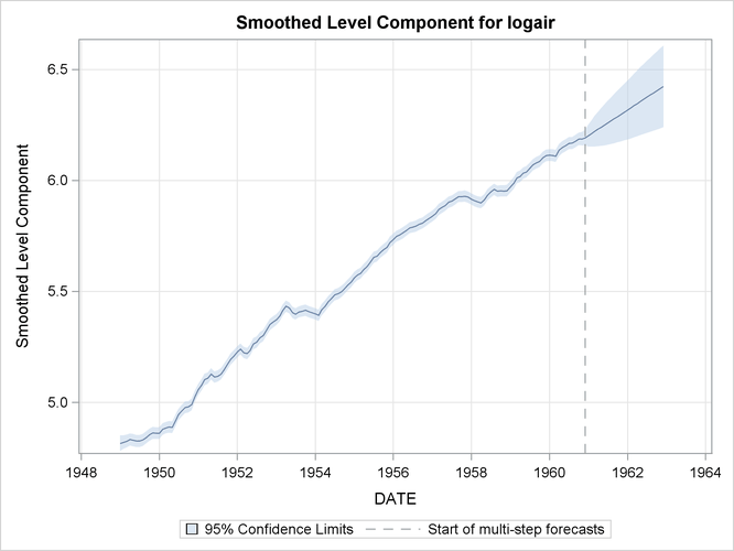
The first plot, shown in Figure 34.5, is produced by the PLOT=SMOOTH option in the LEVEL statement, it shows the smoothed level of the series.
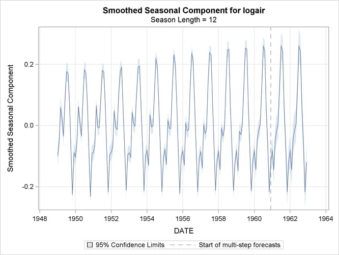
The second plot (Figure 34.6), produced by the PLOT=SMOOTH option in the SEASON statement, shows the smoothed seasonal component by itself.
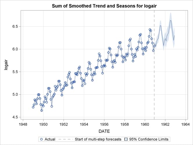
The plot of the sum of the trend and seasonal component, produced by the PLOT=DECOMP option in the FORECAST statement, is shown in Figure 34.7. You can see that, at least visually, the model seems to fit the data well. In all these decomposition plots the component estimates are extrapolated for two years in the future based on the LEAD=24 option specified in the FORECAST statement.