The UCM Procedure
- Overview
-
Getting Started

-
SyntaxFunctional SummaryPROC UCM StatementAUTOREG StatementBLOCKSEASON StatementBY StatementCYCLE StatementDEPLAG StatementESTIMATE StatementFORECAST StatementID StatementIRREGULAR StatementLEVEL StatementMODEL StatementNLOPTIONS StatementOUTLIER StatementPERFORMANCE StatementRANDOMREG StatementSEASON StatementSLOPE StatementSPLINEREG StatementSPLINESEASON Statement
-
Details
-
Examples
- References
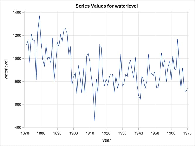
The series in this example consists of the yearly water level readings of the Nile River recorded at Aswan, Egypt (Cobb, 1978; de Jong and Penzer, 1998). The readings are from the years 1871 to 1970. The series does not show any apparent trend or any other distinctive patterns; however, there is a shift in the water level starting at the year 1899. This shift could be attributed to the start of construction of a dam near Aswan in that year. A time series plot of this series is given in Output 34.7.1. The following DATA step statements create the input data set.
data nile;
   input waterlevel @@;
   year = intnx( 'year', '1jan1871'd, _n_-1 );
   format year year4.;
datalines;
   1120  1160  963  1210  1160  1160  813  1230   1370  1140
   995   935   1110 994   1020  960   1180 799    958   1140
   1100  1210  1150 1250  1260  1220  1030 1100   774   840
   874   694   940  833   701   916   692  1020   1050  969
   831   726   456  824   702   1120  1100 832    764   821
   768   845   864  862   698   845   744  796    1040  759
   781   865   845  944   984   897   822  1010   771   676
   649   846   812  742   801   1040  860  874    848   890
   744   749   838  1050  918   986   797  923    975   815
   1020  906   901  1170  912   746   919  718    714   740
;
proc timeseries data=nile plot=series;
   id year interval=year;
   var waterlevel;
run;
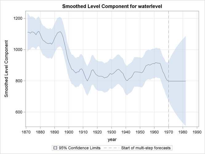
In this situation it is known that a shift in the water level occurred within the span of the series, and its effect can be easily taken into account by including an appropriate indicator variable as a regressor. However, in many situation such prior information is not available, and it is useful to detect such a shift in a data analytic fashion. You can check for breaks in the level by using the CHECKBREAK option in the LEVEL statement. The following statements fit a simple locally constant level plus error model to the series:
proc ucm data=nile;
   id year interval=year;
   model waterlevel;
   irregular;
   level plot=smooth checkbreak;
   estimate;
   forecast plot=decomp;
run;
The plot in Output 34.7.2 shows a noticeable drop in the smoothed water level around 1899.
The “Outlier Summary” table in Output 34.7.3 shows the most likely types of breaks and their locations within the series span. The shift of 1899 is easily detected.
Output 34.7.3: Detection of Structural Breaks in the Nile River Level
| Outlier Summary | |||||||
|---|---|---|---|---|---|---|---|
| Obs | year | Break Type | Estimate | Standard Error | Chi-Square | DF | Pr > ChiSq |
| 29 | 1899 | Level | -315.73791 | 97.639753 | 10.46 | 1 | 0.0012 |
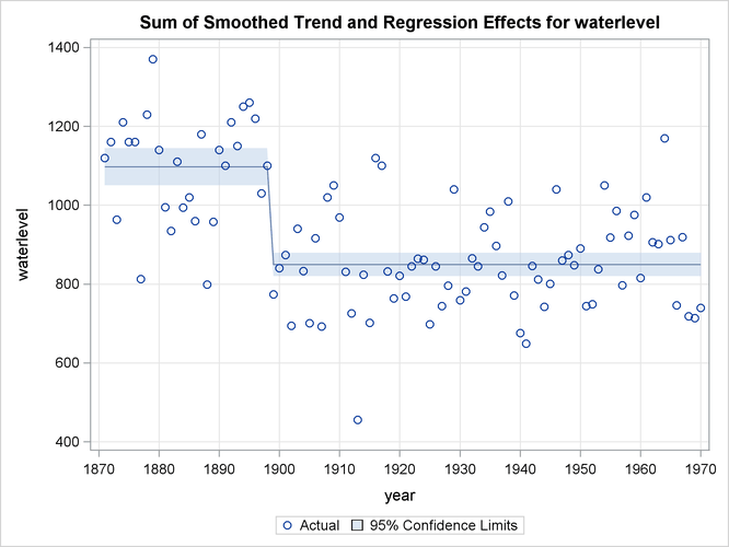
The following statements specify a UCM that models the level of the river as a locally constant series with a shift in the year 1899, represented by a dummy regressor (SHIFT1899):
data nile;
   set nile;
   shift1899 = ( year >= '1jan1899'd );
run;
proc ucm data=nile;
   id year interval=year;
   model waterlevel = shift1899;
   irregular;
   level;
   estimate;
   forecast plot=decomp;
run;
The plot in Output 34.7.4 shows the smoothed trend, including the correction due to the shift in the year 1899. Notice the simplicity in the shape of the smoothed curve after the incorporation of the shift information.