The SSM Procedure
-
Overview

- Getting Started
-
Syntax
-
DetailsState Space Model and NotationTypes of Sequence DataOverview of Model Specification SyntaxFiltering, Smoothing, Likelihood, and Structural Break DetectionEstimation of User-Specified Linear Combination of State ElementsContrasting PROC SSM with Other SAS Procedures Predefined Trend ModelsPredefined Structural ModelsCovariance ParameterizationMissing ValuesComputational IssuesDisplayed OutputODS Table NamesODS Graph NamesOUT= Data Set
-
ExamplesBivariate Basic Structural Model Panel Data: Two-Way Random-Effects and Autoregressive ModelsBackcasting, Forecasting, and InterpolationLongitudinal Data: Smoothing of Repeated MeasuresA User-Defined Trend ModelModel with Multiple ARIMA ComponentsDynamic Factor ModelingDiagnostic Plots and Structural Break AnalysisLongitudinal Data: Variable Bandwidth SmoothingA Transfer Function Model for the Gas Furnace DataPanel Data: Dynamic Panel Model for the Cigar DataMultivariate Modeling: Analysis of Long-Term Temperature Trends
- References
The STATE statement option TYPE=CYCLE(CT) specifies a two-dimensional ![]() , needed for defining a univariate continuous time cycle. In this case the nominal dimension, dim, must be 1. In particular,
, needed for defining a univariate continuous time cycle. In this case the nominal dimension, dim, must be 1. In particular, ![]() becomes one-dimensional, which is denoted by
becomes one-dimensional, which is denoted by ![]() . This cycle can be used for any data type. As before, the parameters of the cycle are a damping factor
. This cycle can be used for any data type. As before, the parameters of the cycle are a damping factor ![]() ,
, ![]() , and period
, and period ![]() . Unlike in the discrete-time cycle described in the section Multivariate Cycle, the period is not required to be larger than 2. Let
. Unlike in the discrete-time cycle described in the section Multivariate Cycle, the period is not required to be larger than 2. Let ![]() , and let
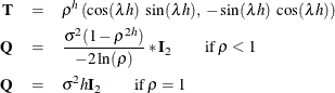
, and let ![]() denote the difference between successive time points. In this case, the system matrices
denote the difference between successive time points. In this case, the system matrices ![]() and
and ![]() that govern
that govern ![]() depend on
depend on ![]() . They are:
. They are:
If ![]() , the initial condition is nondiffuse:
, the initial condition is nondiffuse: ![]() . For
. For ![]() , the initial condition is fully diffuse.
, the initial condition is fully diffuse.
The first element of ![]() corresponds to the needed cycle, and the second element is an auxiliary quantity. You can define a cycle term based on this
state as follows:
corresponds to the needed cycle, and the second element is an auxiliary quantity. You can define a cycle term based on this
state as follows:
     state cycleState(1) type=cycle(CT)  ...;
     component cycle = cycleState[1];
The CT option must be included in the use of TYPE=CYCLE.