The QLIM Procedure
- Overview
-
Getting Started

-
Syntax
-
DetailsOrdinal Discrete Choice ModelingLimited Dependent Variable ModelsStochastic Frontier Production and Cost ModelsHeteroscedasticity and Box-Cox TransformationBivariate Limited Dependent Variable ModelingSelection ModelsMultivariate Limited Dependent ModelsVariable SelectionTests on ParametersEndogeneity and Instrumental VariablesBayesian AnalysisPrior DistributionsOutput to SAS Data SetOUTEST= Data SetNamingODS Table NamesODS Graphics
-
Examples
- References
The PROC QLIM models such as qualitative response or limited dependent variable models assume that the errors are independent of the explanatory variables. If this assumption fails to hold, the distributional form that the likelihood is based on is misspecified and the obtained coefficients are inconsistent.
To begin, consider a linear model
Assume that ![]() ,
, ![]() for
for ![]() , and
, and ![]() . Therefore,
. Therefore, ![]() is endogenous. The endogeneity comes from many sources, such as
is endogenous. The endogeneity comes from many sources, such as ![]() having measurement error or omitting a variable that is correlated with
having measurement error or omitting a variable that is correlated with ![]() . If you ignore the endogeneity, you can estimate this model in PROC QLIM as follows (assuming
. If you ignore the endogeneity, you can estimate this model in PROC QLIM as follows (assuming ![]() ):
):
   proc qlim data=a;
      model y = x1 x2 x3 x4;
   run;
However, this approach produces inconsistent maximum likelihood estimates. To obtain consistent maximum likelihood estimates,
you should consider the joint density of the dependent variable and the endogenous variables. To do this in PROC QLIM, you
need at least one instrument—that is, an observable variable, ![]() —that is not in the structural equation and that satisfies two conditions:
—that is not in the structural equation and that satisfies two conditions: ![]() is exogenous (that is,
is exogenous (that is, ![]() ), and
), and ![]() must be correlated with the endogenous regressor
must be correlated with the endogenous regressor ![]() . Then, you can model
. Then, you can model ![]() as
as
You can now write this reduced form equation along with the structural equation to obtain the consistent maximum likelihood estimates as follows:
   proc qlim data=a;
      model y = x1 x2 x3 x4;
      model x4 = x1 x2 x3 z1;
   run;
Estimating the structural model together with the reduced form models for the endogenous explanatory variables gives you the full information maximum likelihood (FIML) estimates. Because of the linearity of the model, you can estimate it efficiently and more simply by using the two-stage least squares estimator. However, PROC QLIM handles nonlinear models such as qualitative response and limited dependent variable models, and in their estimation it maximizes the corresponding joint likelihood function. In the case of endogeneity, when the reduced form models for the endogenous explanatory variables are written along with the structural model, PROC QLIM maximizes the likelihood function that is obtained from the joint density of the response variable and the endogenous explanatory variables. For example, consider the following censored regression model in which one of the explanatory variables is a continuous endogenous variable:
The exogenous explanatory variables are ![]() , and the continuous endogenous explanatory variable is
, and the continuous endogenous explanatory variable is ![]() .
.
The likelihood function to maximize is
where ![]() is the joint density of
is the joint density of ![]() and
and ![]() . Note that
. Note that ![]() is substituted for
is substituted for ![]() when
when ![]() . If you assume
. If you assume ![]() with
with ![]() , then, by using
, then, by using ![]() , you can write the likelihood function for each
, you can write the likelihood function for each ![]() as a multiplication of two parts. The first part is the probability density function of the normal distribution with mean
as a multiplication of two parts. The first part is the probability density function of the normal distribution with mean
![]() and variance
and variance ![]() , and the second part follows a Tobit model that has latent mean
, and the second part follows a Tobit model that has latent mean ![]() and variance
and variance ![]() . Then, you can obtain the log-likelihood function by taking the log of this multiplication and summing over
. Then, you can obtain the log-likelihood function by taking the log of this multiplication and summing over ![]() (for more information, see Wooldridge (2002, chapter 16)). This is the log-likelihood function that PROC QLIM maximizes.
The parameters
(for more information, see Wooldridge (2002, chapter 16)). This is the log-likelihood function that PROC QLIM maximizes.
The parameters ![]() that are obtained from this maximization are the FIML estimators. Assuming that the latent model includes two instrumental
variables and two exogenous explanatory variables, you can estimate this model in PROC QLIM as follows:
that are obtained from this maximization are the FIML estimators. Assuming that the latent model includes two instrumental
variables and two exogenous explanatory variables, you can estimate this model in PROC QLIM as follows:
   proc qlim data=a;
      model y1 = y2 z11 z12 / censored(lb=0);
      model y2 = z11 z12 z21 z22;
   run;
For simple examples like the preceding ones, you can derive the likelihood function easily. However, as the number of endogenous explanatory variables increases, if these variables have a discontinuous nature, if simultaneity among equations exists, or if a combination of these occurs, then the derivation of the likelihood function becomes cumbersome, or, in some cases, the likelihood function does not even have a closed analytical form.
PROC QLIM can handle endogeneity regardless of the nature of the endogenous explanatory variables for a single structural model. In the case of one endogenous explanatory variable, PROC QLIM reports the FIML estimates that are calculated by using the analytical likelihood function that is obtained from the joint distribution of the dependent variable and the endogenous variable. When there is more than one endogenous explanatory variable, the analytical form of the likelihood function is usually not available; in this case PROC QLIM reports the simulated maximum likelihood estimates. For the simulated maximum likelihood estimation method, PROC QLIM uses the Geweke-Hajivassiliou-Keane (GHK) simulator (see, among others, Hajivassiliou, McFadden, and Ruud (1996)) to simulate the joint distribution of the dependent variable and the endogenous variables. The simulation is facilitated by assuming that the error terms in the latent models for the dependent variable and the endogenous explanatory variables are distributed as multivariate normal.
When you estimate a model in PROC QLIM, you can take the endogeneity into account by writing the structural model along with the reduced form models for each endogenous variable. Examples are provided in the following sections.
Probit Model with a Continuous Endogenous Explanatory Variable
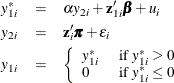
Consider a probit model that contains a single endogenous explanatory variable in addition to two instruments and two exogenous explanatory variables. The model is
where ![]() . You can estimate this model by using the following statements:
. You can estimate this model by using the following statements:
   proc qlim data=a;
      model y1 = y2 z1 z2 / discrete;
      model y2 = z1 z2 z3 z4;
   run;
Probit Model with a Binary Endogenous Explanatory Variable
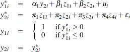
Consider a probit model that contains a single binary endogenous explanatory variable in addition to two instruments and two exogenous explanatory variables. The model is
where ![]() . You can estimate this model by using the following statements:
. You can estimate this model by using the following statements:
   proc qlim data=a;
      model y1 = y2 z1 z2 / discrete;
      model y2 = z1 z2 z3 z4 / discrete;
   run;
Probit Model with a Censored Endogenous Explanatory Variable
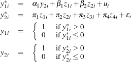
Consider a probit model that contains a single censored (below zero) endogenous explanatory variable in addition to two instruments and two exogenous explanatory variables. The model is
where ![]() . You can estimate this model by using the following statements:
. You can estimate this model by using the following statements:
   proc qlim data=a;
      model y1 = y2 z1 z2 / discrete;
      model y2 = z1 z2 z3 z4 / censored(lb=0);
   run;
Censored Regression Model with a Binary Endogenous Explanatory Variable
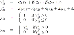
Consider a Type 1 Tobit model that contains a single binary endogenous explanatory variable in addition to two instruments and two exogenous explanatory variables. The model is
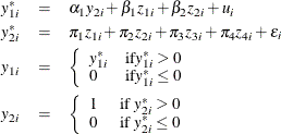
where ![]() . You can estimate this model by using the following statements:
. You can estimate this model by using the following statements:
   proc qlim data=a;
      model y1 = y2 z1 z2 / censored(lb=0);
      model y2 = z1 z2 z3 z4 / discrete;
   run;
Censored Regression Model with Binary and Continuous Endogenous Explanatory Variables
Consider a Type 1 Tobit model that contain binary and continuous endogenous explanatory variables in addition to two instruments and two exogenous explanatory variables. The model is
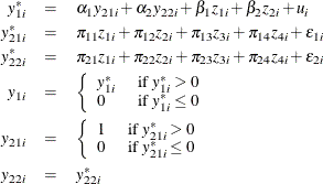
where ![]() . You can estimate this model by using the following statements:
. You can estimate this model by using the following statements:
   proc qlim data=a;
      model y1 = y21 y22 z1 z2 / censored(lb=0);
      model y21 = z1 z2 z3 z4  / discrete;
      model y22 = z1 z2 z3 z4;
   run;
Probit Model with Binary, Censored, and Truncated Endogenous Explanatory Variables
Consider a probit model that contains binary, censored (below zero), and truncated (below zero) endogenous explanatory variables. The model is
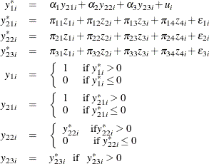
where ![]() are the instrumental variables that are independent of the errors. You can estimate this model by using the following statements:
are the instrumental variables that are independent of the errors. You can estimate this model by using the following statements:
   proc qlim data=a;
      model y1  = y21 y22 y23 / discrete;
      model y21 = z1 z2 z3 z4 / discrete;
      model y22 = z1 z2 z3 z4 / censored(lb=0);
      model y23 = z1 z2 z3 z4 / truncated(lb=0);
   run;
Note that the dependent variable ![]() should not occur in the models for the endogenous explanatory variables, because this causes inconsistent coefficient estimates.
In other words, you should write the models for the endogenous explanatory variables as reduced form models. PROC QLIM does
not handle simultaneous equations models.
should not occur in the models for the endogenous explanatory variables, because this causes inconsistent coefficient estimates.
In other words, you should write the models for the endogenous explanatory variables as reduced form models. PROC QLIM does
not handle simultaneous equations models.
PROC QLIM has two ways to test the null hypothesis that an endogenous explanatory variable (EEV) is in fact exogenous. In
the case of a single EEV, the first testing method involves a likelihood ratio test of ![]() . For example, consider the probit model with a binary endogenous explanatory variable that was considered earlier;
. For example, consider the probit model with a binary endogenous explanatory variable that was considered earlier; ![]() is exogenous if the error term in the model for
is exogenous if the error term in the model for ![]() is uncorrelated with the error term in the model for
is uncorrelated with the error term in the model for ![]() . Therefore, testing to determine whether this correlation is 0 or not provides an endogeneity test for
. Therefore, testing to determine whether this correlation is 0 or not provides an endogeneity test for ![]() . You can do this in PROC QLIM as follows:
. You can do this in PROC QLIM as follows:
   proc qlim data=a;
      model y1 = y2 z1 z2 / discrete;
      model y2 = z1 z2 z3 z4 / discrete;
      test  _rho = 0 / LR;
   run;
Failing to reject the null hypothesis favors the decision that ![]() is exogenous in the model for
is exogenous in the model for ![]() .
.
When there are two or more EEVs, the test becomes the joint likelihood ratio test of whether corresponding correlations are 0 or not.
The second testing method is similar to the approach of Rivers and Vuong (1988). Considering the same model, you can write
where ![]() and
and ![]() is independent of
is independent of ![]() s and
s and ![]() . You can now write
. You can now write
Testing ![]() is the same as testing whether
is the same as testing whether ![]() is correlated with
is correlated with ![]() or testing whether
or testing whether ![]() is endogenous or not. Because
is endogenous or not. Because ![]() are unobserved, you can replace them with the OLS residuals from the model for
are unobserved, you can replace them with the OLS residuals from the model for ![]() and apply a robust t test. Note that even though
and apply a robust t test. Note that even though ![]() is binary (or censored), the test is still correct under
is binary (or censored), the test is still correct under ![]() .
.
This approach can be summarized as a two-step procedure. In the first step, generated regressors—that is, the OLS residuals from the models for each of the EEVs—are obtained. In the second step, the structural model that includes the generated regressors as additional explanatory variables is estimated by the maximum likelihood method and the joint significance of these generated regressors is tested by the Wald test.
In PROC QLIM, you can apply the second method for the same test that was considered previously as follows:
   proc qlim data=a;
      model y1 = y2 z1 z2 / discrete endotest(y2);
      model y2 = z1 z2 z3 z4 / discrete;
   run;
In PROC QLIM you can test the validity of instrumental variables (IVs) by specifying the OVERID option in the ENDOGENOUS
or MODEL statement. The OVERID test is a maximum likelihood version of the overidentifying restrictions test in the IV framework.
If you have more IVs than are necessary for identification—that is, overidentifying IVs—you can use them to test the validity
of your IVs. When you use the OVERID option to specify the overidentifying IVs, it applies the likelihood ratio test of the
joint significance of these IVs, included as additional explanatory variables in the structural model that it estimates by
the MLE jointly with the reduced form models. In effect, you test whether the overidentifying IVs are correlated with the
error term in the structural model. You specify the reduced form models through the overidentifying IVs. The structural model
is the model that includes the OVERID option. For example, consider the probit model that contains a continuous endogenous
explanatory variable. You can consider ![]() or
or ![]() in the model for
in the model for ![]() as an overidentifying IV; therefore, you can specify the OVERID test as follows:
as an overidentifying IV; therefore, you can specify the OVERID test as follows:
   proc qlim data=a;
      model y1 = y2 z1 z2 / discrete overid(y2.z4);
      model y2 = z1 z2 z3 z4;
   run;
In this case, PROC QLIM estimates the structural model ![]() , including the overidentifying IV
, including the overidentifying IV ![]() as an additional explanatory variable in this model, jointly with the reduced form model
as an additional explanatory variable in this model, jointly with the reduced form model ![]() . Then it uses the likelihood ratio test to test the hypothesis that the overidentifying IV is insignificant. Rejecting this
hypothesis raises doubts about the validity of the instruments
. Then it uses the likelihood ratio test to test the hypothesis that the overidentifying IV is insignificant. Rejecting this
hypothesis raises doubts about the validity of the instruments ![]() and
and ![]() .
.
Note that, as long as you have continuous endogenous explanatory variables, the test result is invariant to which overidentifying IVs you specify in the test.