The QLIM Procedure
- Overview
-
Getting Started

-
Syntax
-
DetailsOrdinal Discrete Choice ModelingLimited Dependent Variable ModelsStochastic Frontier Production and Cost ModelsHeteroscedasticity and Box-Cox TransformationBivariate Limited Dependent Variable ModelingSelection ModelsMultivariate Limited Dependent ModelsVariable SelectionTests on ParametersEndogeneity and Instrumental VariablesBayesian AnalysisPrior DistributionsOutput to SAS Data SetOUTEST= Data SetNamingODS Table NamesODS Graphics
-
Examples
- References
When the dependent variable is censored, values in a certain range are all transformed to a single value. For example, the standard tobit model can be defined as
where ![]() . The log-likelihood function of the standard censored regression model is
. The log-likelihood function of the standard censored regression model is
where ![]() is the cumulative density function of the standard normal distribution and
is the cumulative density function of the standard normal distribution and ![]() is the probability density function of the standard normal distribution.
is the probability density function of the standard normal distribution.
The tobit model can be generalized to handle observation-by-observation censoring. The censored model on both of the lower and upper limits can be defined as
![\[ y_{i} = \left\{ \begin{array}{ll} R_{i} & \mr {if} \; y_{i}^{*} \geq R_{i} \\ y_{i}^{*} & \mr {if} \; L_{i} < y_{i}^{*} < R_{i} \\ L_{i} & \mr {if} \; y_{i}^{*} \leq L_{i} \end{array} \right. \]](images/etsug_qlim0130.png)
The log-likelihood function can be written as
![\begin{eqnarray*} \ell & = & \sum _{i\in \{ L_{i}< y_{i} < R_{i}\} } \ln \left[\phi (\frac{y_{i}-\mathbf{x}_{i}\bbeta }{\sigma })/\sigma \right] + \sum _{i\in \{ y_{i}=R_{i}\} } \ln \left[\Phi (-\frac{R_{i}-\mathbf{x}_{i}\bbeta }{\sigma })\right] + \\ & & \sum _{i\in \{ y_{i}=L_{i}\} } \ln \left[\Phi (\frac{L_{i}-\mathbf{x}_{i}\bbeta }{\sigma })\right] \end{eqnarray*}](images/etsug_qlim0131.png)
Log-likelihood functions of the lower- or upper-limit censored model are easily derived from the two-limit censored model. The log-likelihood function of the lower-limit censored model is
The log-likelihood function of the upper-limit censored model is
Amemiya (1984) classified Tobit models into five types based on characteristics of the likelihood function. For notational convenience,
let ![]() denote a distribution or density function,
denote a distribution or density function, ![]() is assumed to be normally distributed with mean
is assumed to be normally distributed with mean ![]() and variance
and variance ![]() .
.
Type 1 Tobit
The Type 1 Tobit model was already discussed in the preceding section.
The likelihood function is characterized as ![]() .
.
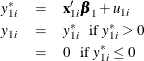
Type 2 Tobit
The Type 2 Tobit model is defined as
where ![]() . The likelihood function is described as
. The likelihood function is described as ![]() .
.
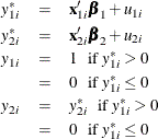
Type 3 Tobit
The Type 3 Tobit model is different from the Type 2 Tobit in that ![]() of the Type 3 Tobit is observed when
of the Type 3 Tobit is observed when ![]() .
.
where ![]() .
.
The likelihood function is characterized as ![]() .
.
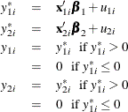
Type 4 Tobit
The Type 4 Tobit model consists of three equations:
where ![]() . The likelihood function of the Type 4 Tobit model is characterized as
. The likelihood function of the Type 4 Tobit model is characterized as ![]() .
.
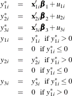
Type 5 Tobit
The Type 5 Tobit model is defined as follows:
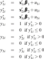
where ![]() are from iid trivariate normal distribution. The likelihood function of the Type 5 Tobit model is characterized as
are from iid trivariate normal distribution. The likelihood function of the Type 5 Tobit model is characterized as ![]() .
.
Code examples for these models can be found in Types of Tobit Models.
In a truncated model, the observed sample is a subset of the population where the dependent variable falls in a certain range.
For example, when neither a dependent variable nor exogenous variables are observed for ![]() , the truncated regression model can be specified.
, the truncated regression model can be specified.
Two-limit truncation model is defined as
The log-likelihood function of the two-limit truncated regression model is
The log-likelihood functions of the lower- and upper-limit truncation model are
![\begin{eqnarray*} \ell & = & \sum _{i=1}^{N}\left\{ \ln \left[\phi (\frac{y_{i}-\mb {x}_{i}\bbeta }{\sigma }) / \sigma \right] - \ln \left[1 - \Phi (\frac{L_{i}-\mb {x}_{i}\bbeta }{\sigma })\right] \right\} \; \; \textrm{(lower)} \\ \ell & = & \sum _{i=1}^{N}\left\{ \ln \left[\phi (\frac{y_{i}-\mb {x}_{i}\bbeta }{\sigma }) / \sigma \right] - \ln \left[\Phi (\frac{R_{i}-\mb {x}_{i}\bbeta }{\sigma })\right] \right\} \; \; \textrm{(upper)} \end{eqnarray*}](images/etsug_qlim0158.png)