The FORECAST Procedure
- Overview
-
Getting Started
 Giving Dates to Forecast ValuesComputing Confidence LimitsForm of the OUT= Data SetPlotting ForecastsPlotting ResidualsModel Parameters and Goodness-of-Fit StatisticsControlling the Forecasting MethodIntroduction to Forecasting MethodsTime Trend ModelsTime Series MethodsCombining Time Trend with Autoregressive Models
 -
Syntax
-
Details
-
Examples
- References
Example 16.2 Forecasting Retail Sales
This example uses the stepwise autoregressive method to forecast the monthly U. S. sales of durable goods (DURABLES) and nondurable goods (NONDUR) from the SASHELP.USECON data set. The data are from Business Statistics, published by the U.S. Bureau of Economic Analysis. The following statements plot the series:
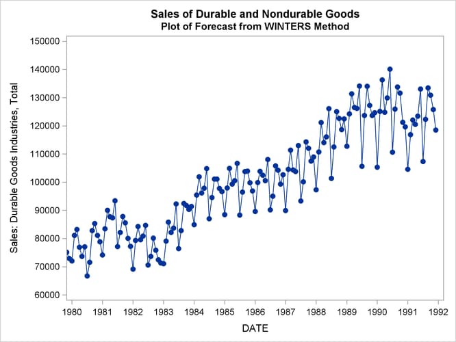
title1 'Sales of Durable and Nondurable Goods';
title2 'Plot of Forecast from WINTERS Method';
proc sgplot data=sashelp.usecon;
   series x=date y=durables / markers markerattrs=(symbol=circlefilled);
   xaxis values=('1jan80'd to '1jan92'd by year);
   yaxis values=(60000 to 150000 by 10000);
   format date year4.;
run;
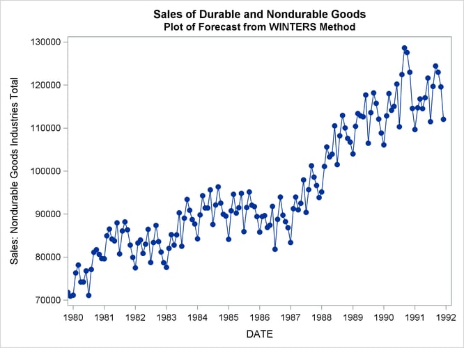
title1 'Sales of Durable and Nondurable Goods';
title2 'Plot of Forecast from WINTERS Method';
proc sgplot data=sashelp.usecon;
   series x=date y=nondur / markers markerattrs=(symbol=circlefilled);
   xaxis values=('1jan80'd to '1jan92'd by year);
   yaxis values=(70000 to 130000 by 10000);
   format date year4.;
run;
The plots are shown in Output 16.2.1 and Output 16.2.2.
Output 16.2.1: Durable Goods Sales
Output 16.2.2: Nondurable Goods Sales
The following statements produce the forecast:
title1 "Forecasting Sales of Durable and Nondurable Goods";

proc forecast data=sashelp.usecon interval=month
              method=stepar trend=2 lead=12
              out=out outfull outest=est;
   id date;
   var durables nondur;
   where date >= '1jan80'd;
run;
The following statements print the OUTEST= data set.
title2 'OUTEST= Data Set: STEPAR Method';
proc print data=est;
run;
The PROC PRINT listing of the OUTEST= data set is shown in Output 16.2.3.
Output 16.2.3: The OUTEST= Data Set Produced by PROC FORECAST
| Forecasting Sales of Durable and Nondurable Goods |
| OUTEST= Data Set: STEPAR Method |
| Obs | _TYPE_ | DATE | DURABLES | NONDUR |
|---|---|---|---|---|
| 1 | N | DEC91 | 144 | 144 |
| 2 | NRESID | DEC91 | 144 | 144 |
| 3 | DF | DEC91 | 137 | 139 |
| 4 | SIGMA | DEC91 | 4519.451 | 2452.2642 |
| 5 | CONSTANT | DEC91 | 71884.597 | 73190.812 |
| 6 | LINEAR | DEC91 | 400.90106 | 308.5115 |
| 7 | AR01 | DEC91 | 0.5844515 | 0.8243265 |
| 8 | AR02 | DEC91 | . | . |
| 9 | AR03 | DEC91 | . | . |
| 10 | AR04 | DEC91 | . | . |
| 11 | AR05 | DEC91 | . | . |
| 12 | AR06 | DEC91 | 0.2097977 | . |
| 13 | AR07 | DEC91 | . | . |
| 14 | AR08 | DEC91 | . | . |
| 15 | AR09 | DEC91 | . | . |
| 16 | AR10 | DEC91 | -0.119425 | . |
| 17 | AR11 | DEC91 | . | . |
| 18 | AR12 | DEC91 | 0.6138699 | 0.8050854 |
| 19 | AR13 | DEC91 | -0.556707 | -0.741854 |
| 20 | SST | DEC91 | 4.923E10 | 2.8331E10 |
| 21 | SSE | DEC91 | 1.88157E9 | 544657337 |
| 22 | MSE | DEC91 | 13734093 | 3918398.1 |
| 23 | RMSE | DEC91 | 3705.9538 | 1979.4944 |
| 24 | MAPE | DEC91 | 2.9252601 | 1.6555935 |
| 25 | MPE | DEC91 | -0.253607 | -0.085357 |
| 26 | MAE | DEC91 | 2866.675 | 1532.8453 |
| 27 | ME | DEC91 | -67.87407 | -29.63026 |
| 28 | RSQUARE | DEC91 | 0.9617803 | 0.9807752 |
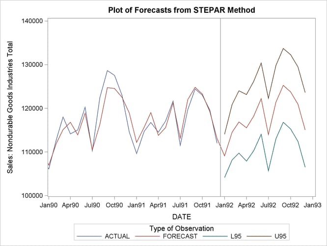
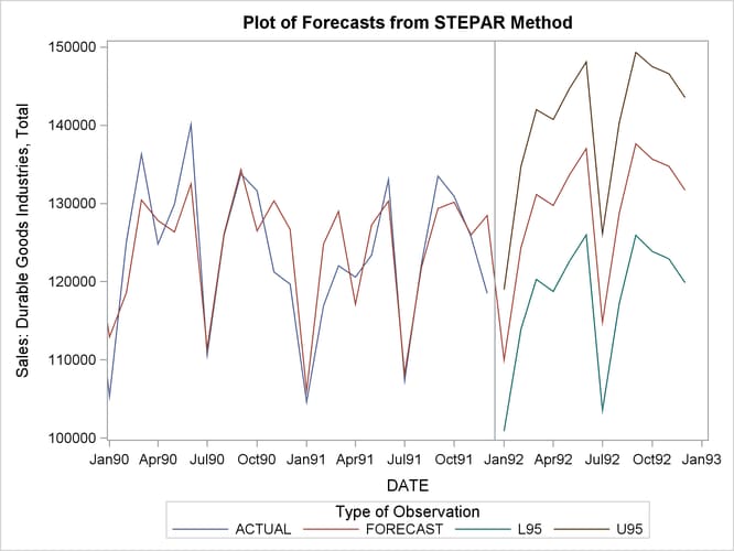
The following statements plot the forecasts and confidence limits. The last two years of historical data are included in the plots to provide context for the forecast. A reference line is drawn at the start of the forecast period.
title1 'Plot of Forecasts from STEPAR Method';
proc sgplot data=out;
   series x=date y=durables / group=_type_;
   xaxis values=('1jan90'd to '1jan93'd by qtr);
   yaxis values=(100000 to 150000 by 10000);
   refline '15dec91'd / axis=x;
run;
proc sgplot data=out;
   series x=date y=nondur / group=_type_;
   xaxis values=('1jan90'd to '1jan93'd by qtr);
   yaxis values=(100000 to 140000 by 10000);
   refline '15dec91'd / axis=x;
run;
The plots are shown in Output 16.2.4 and Output 16.2.5.
Output 16.2.4: Forecast of Durable Goods Sales
Output 16.2.5: Forecast of Nondurable Goods Sales