The ESM Procedure

This example illustrates how the ESM procedure can be used to forecast transactional data.

The following DATA step creates a data set from data recorded at several Internet Web sites. The data set WEBSITES contains a variable TIME that represents time and the variables ENGINE, BOATS, CARS, and PLANES that represent Internet Web site data. Each value of the TIME variable is recorded in ascending order, and the values of each of the other variables represent a transactional data series.

The following ESM procedure statements forecast each of the transactional data series:

proc esm data=websites out=nextweek lead=7;
   id time interval=dtday accumulate=total;
   forecast boats cars planes;
run;

The preceding statements accumulate the data into a daily time series, generate forecasts for the BOATS, CARS, and PLANES variables in the input data set WEBSITES for the next week, and the forecasts are stored in the OUT= data set NEXTWEEK.

The following statements plot the forecasts related to the Internet data:

title1 "Website Data";
proc sgplot data=nextweek;
   series x=time y=boats / markers 
                           markerattrs=(symbol=circlefilled color=red)
                           lineattrs=(color=red); 
   series x=time y=cars / markers 
                           markerattrs=(symbol=asterisk color=blue)
                           lineattrs=(color=blue);
   series x=time y=planes / markers 
                           markerattrs=(symbol=circle color=styg)
                           lineattrs=(color=styg); 
   refline '11APR2000:00:00:00'dt / axis=x;
   xaxis values=('13MAR2000:00:00:00'dt to '18APR2000:00:00:00'dt by dtweek);
   yaxis label='Websites' minor;
run;

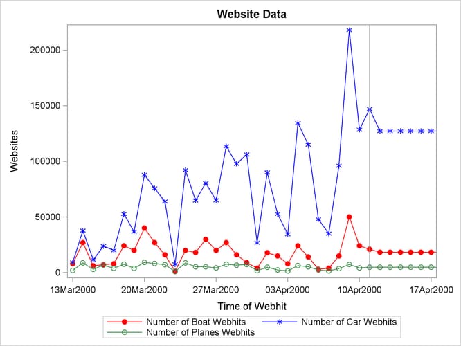
The plots are shown in Output 14.2.1. The historical data is shown to the left of the reference line and the forecasts for the next seven days are shown to the right.