The ARIMA Procedure
- Overview
-
Getting Started
 The Three Stages of ARIMA ModelingIdentification StageEstimation and Diagnostic Checking StageForecasting StageUsing ARIMA Procedure StatementsGeneral Notation for ARIMA ModelsStationarityDifferencingSubset, Seasonal, and Factored ARMA ModelsInput Variables and Regression with ARMA ErrorsIntervention Models and Interrupted Time SeriesRational Transfer Functions and Distributed Lag ModelsForecasting with Input VariablesData Requirements
 -
Syntax
-
DetailsThe Inverse Autocorrelation FunctionThe Partial Autocorrelation FunctionThe Cross-Correlation FunctionThe ESACF MethodThe MINIC MethodThe SCAN MethodStationarity TestsPrewhiteningIdentifying Transfer Function ModelsMissing Values and AutocorrelationsEstimation DetailsSpecifying Inputs and Transfer FunctionsInitial ValuesStationarity and InvertibilityNaming of Model ParametersMissing Values and Estimation and ForecastingForecasting DetailsForecasting Log Transformed DataSpecifying Series PeriodicityDetecting OutliersOUT= Data SetOUTCOV= Data SetOUTEST= Data SetOUTMODEL= SAS Data SetOUTSTAT= Data SetPrinted OutputODS Table NamesStatistical Graphics
-
Examples
- References
Estimation and Diagnostic Checking Stage
The autocorrelation plots for this series, as shown in the previous section, suggest an AR(1) model for the change in SALES. You should check the diagnostic statistics to see if the AR(1) model is adequate. Other candidate models include an MA(1)
model and low-order mixed ARMA models. In this example, the AR(1) model is tried first.
Estimating an AR(1) Model
The following statements fit an AR(1) model (an autoregressive model of order 1), which predicts the change in SALES as an average change, plus some fraction of the previous change, plus a random error. To estimate an AR model, you specify
the order of the autoregressive model with the P= option in an ESTIMATE statement:
   estimate p=1;
   run;
The ESTIMATE statement fits the model to the data and prints parameter estimates and various diagnostic statistics that indicate how well the model fits the data. The first part of the ESTIMATE statement output, the table of parameter estimates, is shown in Figure 7.8.
Figure 7.8: Parameter Estimates for AR(1) Model
| Conditional Least Squares Estimation | |||||
|---|---|---|---|---|---|
| Parameter | Estimate | Standard Error | t Value | Approx Pr > |t| |
Lag |
| MU | 0.90280 | 0.65984 | 1.37 | 0.1744 | 0 |
| AR1,1 | 0.86847 | 0.05485 | 15.83 | <.0001 | 1 |
The table of parameter estimates is titled “Conditional Least Squares Estimation,” which indicates the estimation method used. You can request different estimation methods with the METHOD= option.
The table of parameter estimates lists the parameters in the model; for each parameter, the table shows the estimated value and the standard error and t value for the estimate. The table also indicates the lag at which the parameter appears in the model.
In this case, there are two parameters in the model. The mean term is labeled MU; its estimated value is 0.90280. The autoregressive
parameter is labeled AR1,1; this is the coefficient of the lagged value of the change in SALES, and its estimate is 0.86847.
The t values provide significance tests for the parameter estimates and indicate whether some terms in the model might be unnecessary. In this case, the t value for the autoregressive parameter is 15.83, so this term is highly significant. The t value for MU indicates that the mean term adds little to the model.
The standard error estimates are based on large sample theory. Thus, the standard errors are labeled as approximate, and the standard errors and t values might not be reliable in small samples.
The next part of the ESTIMATE statement output is a table of goodness-of-fit statistics, which aid in comparing this model to other models. This output is shown in Figure 7.9.
Figure 7.9: Goodness-of-Fit Statistics for AR(1) Model
| Constant Estimate | 0.118749 |
|---|---|
| Variance Estimate | 1.15794 |
| Std Error Estimate | 1.076076 |
| AIC | 297.4469 |
| SBC | 302.6372 |
| Number of Residuals | 99 |
The “Constant Estimate” is a function of the mean term MU and the autoregressive parameters. This estimate is computed only for AR or ARMA models, but not for strictly MA models. See the section General Notation for ARIMA Models for an explanation of the constant estimate.
The “Variance Estimate” is the variance of the residual series, which estimates the innovation variance. The item labeled “Std Error Estimate” is the square root of the variance estimate. In general, when you are comparing candidate models, smaller AIC and SBC statistics indicate the better fitting model. The section Estimation Details explains the AIC and SBC statistics.
The ESTIMATE statement next prints a table of correlations of the parameter estimates, as shown in Figure 7.10. This table can help you assess the extent to which collinearity might have influenced the results. If two parameter estimates are very highly correlated, you might consider dropping one of them from the model.
Figure 7.10: Correlations of the Estimates for AR(1) Model
| Correlations of Parameter Estimates |
||
|---|---|---|
| Parameter | MU | AR1,1 |
| MU | 1.000 | 0.114 |
| AR1,1 | 0.114 | 1.000 |
The next part of the ESTIMATE statement output is a check of the autocorrelations of the residuals. This output has the same form as the autocorrelation check for white noise that the IDENTIFY statement prints for the response series. The autocorrelation check of residuals is shown in Figure 7.11.
Figure 7.11: Check for White Noise Residuals for AR(1) Model
| Autocorrelation Check of Residuals | |||||||||
|---|---|---|---|---|---|---|---|---|---|
| To Lag | Chi-Square | DF | Pr > ChiSq | Autocorrelations | |||||
| 6 | 19.09 | 5 | 0.0019 | 0.327 | -0.220 | -0.128 | 0.068 | -0.002 | -0.096 |
| 12 | 22.90 | 11 | 0.0183 | 0.072 | 0.116 | -0.042 | -0.066 | 0.031 | -0.091 |
| 18 | 31.63 | 17 | 0.0167 | -0.233 | -0.129 | -0.024 | 0.056 | -0.014 | -0.008 |
| 24 | 32.83 | 23 | 0.0841 | 0.009 | -0.057 | -0.057 | -0.001 | 0.049 | -0.015 |
The ![]() test statistics for the residuals series indicate whether the residuals are uncorrelated (white noise) or contain additional
information that might be used by a more complex model. In this case, the test statistics reject the no-autocorrelation hypothesis
at a high level of significance (p = 0.0019 for the first six lags.) This means that the residuals are not white noise, and so the AR(1) model is not a fully
adequate model for this series. The ESTIMATE statement output also includes graphical analysis of the residuals. It is not
shown here. The graphical analysis also reveals the inadequacy of the AR(1) model.
test statistics for the residuals series indicate whether the residuals are uncorrelated (white noise) or contain additional
information that might be used by a more complex model. In this case, the test statistics reject the no-autocorrelation hypothesis
at a high level of significance (p = 0.0019 for the first six lags.) This means that the residuals are not white noise, and so the AR(1) model is not a fully
adequate model for this series. The ESTIMATE statement output also includes graphical analysis of the residuals. It is not
shown here. The graphical analysis also reveals the inadequacy of the AR(1) model.
The final part of the ESTIMATE statement output is a listing of the estimated model, using the backshift notation. This output is shown in Figure 7.12.
Figure 7.12: Estimated ARIMA(1, 1, 0) Model for SALES
| Model for variable sales | |
|---|---|
| Estimated Mean | 0.902799 |
| Period(s) of Differencing | 1 |
| Autoregressive Factors | |
|---|---|
| Factor 1: | 1 - 0.86847 B**(1) |
This listing combines the differencing specification given in the IDENTIFY statement with the parameter estimates of the model
for the change in SALES. Since the AR(1) model is for the change in SALES, the final model for SALES is an ARIMA(1,1,0) model. Using ![]() , the backshift operator, the mathematical form of the estimated model shown in this output is as follows:
, the backshift operator, the mathematical form of the estimated model shown in this output is as follows:
|
|
See the section General Notation for ARIMA Models for further explanation of this notation.
Estimating an ARMA(1,1) Model
The IDENTIFY statement plots suggest a mixed autoregressive and moving-average model, and the previous ESTIMATE statement
check of residuals indicates that an AR(1) model is not sufficient. You now try estimating an ARMA(1,1) model for the change
in SALES.
An ARMA(1,1) model predicts the change in SALES as an average change, plus some fraction of the previous change, plus a random error, plus some fraction of the random error
in the preceding period. An ARMA(1,1) model for the change in SALES is the same as an ARIMA(1,1,1) model for the level of SALES.
To estimate a mixed autoregressive moving-average model, you specify the order of the moving-average part of the model with
the Q= option in an ESTIMATE statement in addition to specifying the order of the autoregressive part with the P= option.
The following statements fit an ARMA(1,1) model to the differenced SALES series:
   estimate p=1 q=1;
   run;
The parameter estimates table and goodness-of-fit statistics for this model are shown in Figure 7.13.
Figure 7.13: Estimated ARMA(1, 1) Model for Change in SALES
| Conditional Least Squares Estimation | |||||
|---|---|---|---|---|---|
| Parameter | Estimate | Standard Error | t Value | Approx Pr > |t| |
Lag |
| MU | 0.89288 | 0.49391 | 1.81 | 0.0738 | 0 |
| MA1,1 | -0.58935 | 0.08988 | -6.56 | <.0001 | 1 |
| AR1,1 | 0.74755 | 0.07785 | 9.60 | <.0001 | 1 |
| Constant Estimate | 0.225409 |
|---|---|
| Variance Estimate | 0.904034 |
| Std Error Estimate | 0.950807 |
| AIC | 273.9155 |
| SBC | 281.7009 |
| Number of Residuals | 99 |
The moving-average parameter estimate, labeled “MA1,1”, is –0.58935. Both the moving-average and the autoregressive parameters have significant t values. Note that the variance estimate, AIC, and SBC are all smaller than they were for the AR(1) model, indicating that the ARMA(1,1) model fits the data better without over-parameterizing.
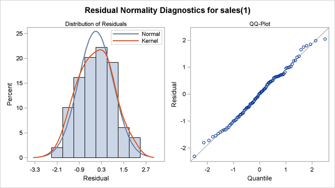
The graphical check of the residuals from this model is shown in Figure 7.14 and Figure 7.15. The residual correlation and white noise test plots show that you cannot reject the hypothesis that the residuals are uncorrelated.
The normality plots also show no departure from normality. Thus, you conclude that the ARMA(1,1) model is adequate for the
change in SALES series, and there is no point in trying more complex models.
Figure 7.14: White Noise Check of Residuals for the ARMA(1,1) Model
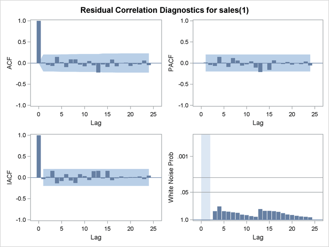
Figure 7.15: Normality Check of Residuals for the ARMA(1,1) Model
The form of the estimated ARIMA(1,1,1) model for SALES is shown in Figure 7.16.
Figure 7.16: Estimated ARIMA(1,1,1) Model for SALES
| Model for variable sales | |
|---|---|
| Estimated Mean | 0.892875 |
| Period(s) of Differencing | 1 |
| Autoregressive Factors | |
|---|---|
| Factor 1: | 1 - 0.74755 B**(1) |
| Moving Average Factors | |
|---|---|
| Factor 1: | 1 + 0.58935 B**(1) |
The estimated model shown in this output is
|
|
In addition to the residual analysis of a model, it is often useful to check whether there are any changes in the time series that are not accounted for by the currently estimated model. The OUTLIER statement enables you to detect such changes. For a long series, this task can be computationally burdensome. Therefore, in general, it is better done after a model that fits the data reasonably well has been found. Figure 7.17 shows the output of the simplest form of the OUTLIER statement:
   outlier;
   run;
Two possible outliers have been found for the model in question. See the section Detecting Outliers, and the examples Example 7.6 and Example 7.7, for more details about modeling in the presence of outliers. In this illustration these outliers are not discussed any further.
Figure 7.17: Outliers for the ARIMA(1,1,1) Model for SALES
| Outlier Detection Summary | |
|---|---|
| Maximum number searched | 2 |
| Number found | 2 |
| Significance used | 0.05 |
| Outlier Details | ||||
|---|---|---|---|---|
| Obs | Type | Estimate | Chi-Square | Approx Prob>ChiSq |
| 10 | Additive | 0.56879 | 4.20 | 0.0403 |
| 67 | Additive | 0.55698 | 4.42 | 0.0355 |
Since the model diagnostic tests show that all the parameter estimates are significant and the residual series is white noise,
the estimation and diagnostic checking stage is complete. You can now proceed to forecasting the SALES series with this ARIMA(1,1,1) model.