The ARIMA Procedure
- Overview
-
Getting Started
 The Three Stages of ARIMA ModelingIdentification StageEstimation and Diagnostic Checking StageForecasting StageUsing ARIMA Procedure StatementsGeneral Notation for ARIMA ModelsStationarityDifferencingSubset, Seasonal, and Factored ARMA ModelsInput Variables and Regression with ARMA ErrorsIntervention Models and Interrupted Time SeriesRational Transfer Functions and Distributed Lag ModelsForecasting with Input VariablesData Requirements
 -
Syntax
-
DetailsThe Inverse Autocorrelation FunctionThe Partial Autocorrelation FunctionThe Cross-Correlation FunctionThe ESACF MethodThe MINIC MethodThe SCAN MethodStationarity TestsPrewhiteningIdentifying Transfer Function ModelsMissing Values and AutocorrelationsEstimation DetailsSpecifying Inputs and Transfer FunctionsInitial ValuesStationarity and InvertibilityNaming of Model ParametersMissing Values and Estimation and ForecastingForecasting DetailsForecasting Log Transformed DataSpecifying Series PeriodicityDetecting OutliersOUT= Data SetOUTCOV= Data SetOUTEST= Data SetOUTMODEL= SAS Data SetOUTSTAT= Data SetPrinted OutputODS Table NamesStatistical Graphics
-
Examples
- References
Statistical Graphics
Statistical procedures use ODS Graphics to create graphs as part of their output. ODS Graphics is described in detail in Chapter 21: Statistical Graphics Using ODS in SAS/STAT 12.1 User's Guide.
Before you create graphs, ODS Graphics must be enabled (for example, with the ODS GRAPHICS ON statement). For more information about enabling and disabling ODS Graphics, see the section “Enabling and Disabling ODS Graphics” in that chapter.
The overall appearance of graphs is controlled by ODS styles. Styles and other aspects of using ODS Graphics are discussed in the section “A Primer on ODS Statistical Graphics” in that chapter.
This section provides information about the graphics produced by the ARIMA procedure. (See Chapter 21: Statistical Graphics Using ODS in SAS/STAT 12.1 User's Guide, for more information about ODS statistical graphics.) The main types of plots available are as follows:
-
plots useful in the trend and correlation analysis of the dependent and input series
-
plots useful for the residual analysis of an estimated model
-
forecast plots
You can obtain most plots relevant to the specified model by default. For finer control of the graphics, you can use the PLOTS= option in the PROC ARIMA statement. The following example is a simple illustration of how to use the PLOTS= option.
Airline Series: Illustration of ODS Graphics
The series in this example, the monthly airline passenger series, is also discussed later, in Example 7.2.
The following statements specify an ARIMA(0,1,1)![]() (0,1,1)
(0,1,1)![]() model without a mean term to the logarithms of the airline passengers series,
model without a mean term to the logarithms of the airline passengers series, xlog. Notice the use of the global plot option ONLY in the PLOTS= option of the PROC ARIMA statement. It suppresses the production of default graphics and produces only the plots specified
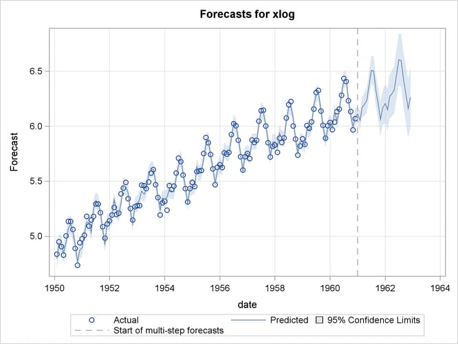
by the subsequent RESIDUAL and FORECAST plot options. The RESIDUAL(SMOOTH) plot specification produces a time series plot of residuals that has an overlaid loess fit; see Figure 7.21. The FORECAST(FORECAST) option produces a plot that shows the one-step-ahead forecasts, as well as the multistep-ahead forecasts; see Figure 7.22.
proc arima data=seriesg
   plots(only)=(residual(smooth) forecast(forecasts));
   identify var=xlog(1,12);
   estimate q=(1)(12) noint method=ml;
   forecast id=date interval=month;
run;
Figure 7.21: Residual Plot of the Airline Model
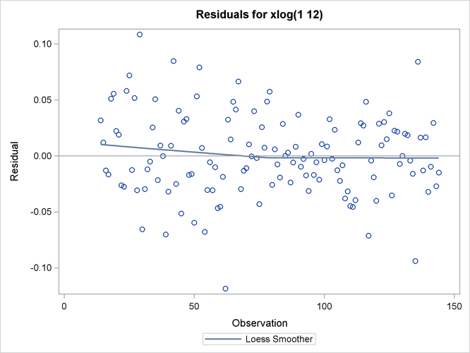
Figure 7.22: Forecast Plot of the Airline Model
ODS Graph Names
PROC ARIMA assigns a name to each graph it creates by using ODS. You can use these names to reference the graphs when you use ODS. The names are listed in Table 7.13.
Table 7.13: ODS Graphics Produced by PROC ARIMA
|
ODS Graph Name |
Plot Description |
Option |
|---|---|---|
|
SeriesPlot |
Time series plot of the dependent series |
|
|
SeriesACFPlot |
Autocorrelation plot of the dependent series |
|
|
SeriesPACFPlot |
Partial-autocorrelation plot of the dependent series |
|
|
SeriesIACFPlot |
Inverse-autocorrelation plot of the dependent series |
|
|
SeriesCorrPanel |
Series trend and correlation analysis panel |
Default |
|
CrossCorrPanel |
Cross-correlation plots, either individual or paneled. They are numbered 1, 2, and so on as needed. |
Default |
|
ResidualACFPlot |
Residual-autocorrelation plot |
|
|
ResidualPACFPlot |
Residual-partial-autocorrelation plot |
|
|
ResidualIACFPlot |
Residual-inverse-autocorrelation plot |
|
|
ResidualWNPlot |
Residual-white-noise-probability plot |
|
|
ResidualHistogram |
Residual histogram |
|
|
ResidualQQPlot |
Residual normal Q-Q Plot |
|
|
ResidualPlot |
Time series plot of residuals with a superimposed smoother |
PLOTS=RESIDUAL(SMOOTH) |
|
ForecastsOnlyPlot |
Time series plot of multistep forecasts |
Default |
|
ForecastsPlot |
Time series plot of one-step-ahead as well as multistep forecasts |
PLOTS=FORECAST(FORECAST) |