The QLIM Procedure
- Overview
-
Getting Started

-
Syntax
-
Details
Ordinal Discrete Choice Modeling Limited Dependent Variable Models Stochastic Frontier Production and Cost Models Heteroscedasticity and Box-Cox Transformation Bivariate Limited Dependent Variable Modeling Selection Models Multivariate Limited Dependent Models Tests on Parameters Output to SAS Data Set OUTEST= Data Set Naming ODS Table Names
-
Examples
- References
| Output to SAS Data Set |
XBeta, Predicted, Residual
Xbeta is the structural part on the right-hand side of the model. Predicted value is the predicted dependent variable value. For censored variables, if the predicted value is outside the boundaries, it is reported as the closest boundary. For discrete variables, it is the level whose boundaries Xbeta falls between. Residual is defined only for continuous variables and is defined as
 |
Error Standard Deviation
Error standard deviation is  in the model. It varies only when the HETERO statement is used.
Marginal Effects
Marginal effect is defined as a contribution of one control variable to the response variable. For the binary choice model with two response categories,  ,
,  , ; and ordinal response model with
  response categories,
  , define
 |
The probability that the unobserved dependent variable is contained in the  th category can be written as
 |
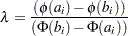
The marginal effect of changes in the regressors on the probability of  is then
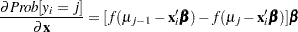 |
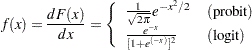
where  . In particular,
 |
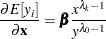
The marginal effects in the Box-Cox regression model are
 |
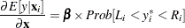
The marginal effects in the truncated regression model are
 |
where  and
and  .
.
The marginal effects in the censored regression model are
 |
Inverse Mills Ratio, Expected and Conditionally Expected Values
Expected and conditionally expected values are computed only for continuous variables. The inverse Mills ratio is computed for censored or truncated continuous, binary discrete, and selection endogenous variables.
Let  and
and  be the lower boundary and upper boundary, respectively, for the
  . Define and . Then the inverse Mills ratio is defined as
 |
for a continuous variable and defined as
 |
for a binary discrete variable.
The expected value is the unconditional expectation of the dependent variable. For a censored variable, it is
 |
For a left-censored variable ( ), this formula is
 |
where  .
.
For a right-censored variable ( ), this formula is
 |
where  .
.
For a noncensored variable, this formula is
 |
The conditional expected value is the expectation given that the variable is inside the boundaries:
 |
Probability
Probability applies only to discrete responses. It is the marginal probability that the discrete response is taking the value of the observation. If the PROBALL option is specified, then the probability for all of the possible responses of the discrete variables is computed.
Technical Efficiency
Technical efficiency for each producer is computed only for stochastic frontier models.
In general, the stochastic production frontier can be written as
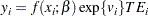 |
where denotes producer  ’s actual output,
  is the deterministic part of production frontier,
  is a producer-specific error term, and
  is the technical efficiency coefficient, which can be written as
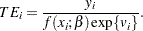 |
In the case of a Cobb-Douglas production function,  . See the section Stochastic Frontier Production and Cost Models.
Cost frontier can be written in general as
 |
where  denotes producer ’s input prices,
  is the deterministic part of cost frontier, is a producer-specific error term, and
  is the cost efficiency coefficient, which can be written as
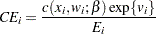 |
In the case of a Cobb-Douglas cost function, 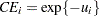 . See the section Stochastic Frontier Production and Cost Models. Hence, both technical and cost efficiency coefficients are the same. The estimates of technical efficiency are provided in the following subsections.
Normal-Half Normal Model
Define  and
and  . Then, as it is shown by Jondrow et al. (1982), conditional density is as follows:
 |
Hence,  is the density for
  .
.
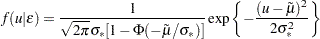
Using this result, it follows that the estimate of technical efficiency (Battese and Coelli, 1988) is
 |
The second version of the estimate (Jondrow et al., 1982) is
 |
where
 |
Normal-Exponential Model
Define  and
and 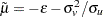 . Then, as it is shown by Kumbhakar and Lovell (2000), conditional density is as follows:
 |
Hence, is the density for  .
.
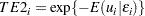
Using this result, it follows that the estimate of technical efficiency is
 |
The second version of the estimate is
|
where
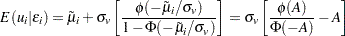 |
Normal-Truncated Normal Model
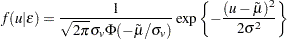
Define 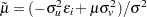 and . Then, as it is shown by Kumbhakar and Lovell (2000), conditional density is as follows:
 |
Hence, is the density for  .
.
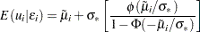
Using this result, it follows that the estimate of technical efficiency is
 |
The second version of the estimate is
|
where
 |