PROC MODEL: OLS Single Nonlinear Equation

Example 19.1 OLS Single Nonlinear Equation

This example illustrates the use of the MODEL procedure for nonlinear ordinary least squares (OLS) regression. The model is a logistic growth curve for the population of the United States. The data is the population in millions recorded at ten-year intervals starting in 1790 and ending in 2000. For an explanation of the starting values given by the START= option, see the section Troubleshooting Convergence Problems. Portions of the output from the following statements are shown in Output 19.1.1 through Output 19.1.3.

title 'Logistic Growth Curve Model of U.S. Population';
data uspop;
   input pop :6.3 @@;
   retain year 1780;
   year=year+10;
   label pop='U.S. Population in Millions';
   datalines;
3929  5308  7239   9638  12866  17069  23191  31443  39818 50155
62947 75994 91972 105710 122775 131669 151325 179323 203211
226542 248710
;

proc model data=uspop;
   label a = 'Maximum Population'
         b = 'Location Parameter'
         c = 'Initial Growth Rate';
   pop = a / ( 1 + exp( b - c * (year-1790) ) );
   fit pop start=(a 1000  b 5.5  c .02) / out=resid outresid;
run;

Output 19.1.1 Logistic Growth Curve Model Summary

Logistic Growth Curve Model of U.S. Population

The MODEL Procedure

Model Summary
Model Variables	1
Parameters	3
Equations	1
Number of Statements	1

Model Variables	pop
Parameters(Value)	a(1000) b(5.5) c(0.02)
Equations	pop

The Equation to Estimate is
pop =	F(a, b, c)

Output 19.1.2 Logistic Growth Curve Estimation Summary

Logistic Growth Curve Model of U.S. Population

The MODEL Procedure

OLS Estimation Summary

Data Set Options
DATA=	USPOP
OUT=	RESID

Minimization Summary
Parameters Estimated	3
Method	Gauss
Iterations	7
Subiterations	6
Average Subiterations	0.857143

Final Convergence Criteria
R	0.00068
PPC(a)	0.000145
RPC(a)	0.001507
Object	0.000065
Trace(S)	19.20198
Objective Value	16.45884

Observations Processed
Read	21
Solved	21

Output 19.1.3 Logistic Growth Curve Estimates

Logistic Growth Curve Model of U.S. Population

The MODEL Procedure

Nonlinear OLS Summary of Residual Errors
Equation	DF Model	DF Error	SSE	MSE	Root MSE	R-Square	Adj R-Sq	Label
pop	3	18	345.6	19.2020	4.3820	0.9972	0.9969	U.S. Population in Millions

Nonlinear OLS Parameter Estimates
Parameter	Estimate	Approx Std Err	t Value	Approx Pr > \|t\|	Label
a	387.9307	30.0404	12.91	<.0001	Maximum Population
b	3.990385	0.0695	57.44	<.0001	Location Parameter
c	0.022703	0.00107	21.22	<.0001	Initial Growth Rate

The adjusted $\text{[math]}$ value indicates the model fits the data well. There are only 21 observations and the model is nonlinear, so significance tests on the parameters are only approximate. The significance tests and associated approximate probabilities indicate that all the parameters are significantly different from 0.

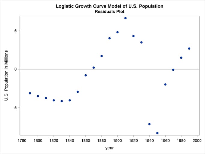
The FIT statement included the options OUT=RESID and OUTRESID so that the residuals from the estimation are saved to the data set RESID. The residuals are plotted to check for heteroscedasticity by using PROC SGPLOT as follows.

title2 "Residuals Plot";
proc sgplot data=resid;
   refline 0;
   scatter x=year y=pop / markerattrs=(symbol=circlefilled);
   xaxis values=(1780 to 2000 by 20);
run;

The plot is shown in Output 19.1.4.

Output 19.1.4 Residual for Population Model (Actual–Predicted)

The residuals do not appear to be independent, and the model could be modified to explain the remaining nonrandom errors.