The ENTROPY Procedure (Experimental)
- Overview
-
Getting Started

-
Syntax
-
Details
Generalized Maximum Entropy Generalized Cross Entropy Moment Generalized Maximum Entropy Maximum Entropy-Based Seemingly Unrelated Regression Generalized Maximum Entropy for Multinomial Discrete Choice Models Censored or Truncated Dependent Variables Information Measures Parameter Covariance For GCE Parameter Covariance For GCE-M Statistical Tests Missing Values Input Data Sets Output Data Sets ODS Table Names ODS Graphics
-
Examples
- References
| Generalized Cross Entropy |
Kullback and Leibler (1951) cross entropy measures the "discrepancy" between one distribution and another. Cross entropy is called a measure of discrepancy rather than distance because it does not satisfy some of the properties one would expect of a distance measure. (See Kapur and Kesavan (1992) for a discussion of cross entropy as a measure of discrepancy.) Mathematically, cross entropy is written as
 |
 |
 |
|||
 |
|
 |
where  is the probability associated with the ith point in the distribution from which the discrepancy is measured. The (in conjunction with the support) are often referred to as the prior distribution. The measure is nonnegative and is equal to zero when
  equals . The properties of the cross entropy measure are examined by Kapur and Kesavan (1992).
The principle of minimum cross entropy (Kullback; 1959; Good; 1963) states that one should choose probabilities that are as close as possible to the prior probabilities. That is, out of all probability distributions that satisfy a given set of constraints which reflect known information about the distribution, choose the distribution that is closest (as measured by  ) to the prior distribution. When the prior distribution is uniform, maximum entropy and minimum cross entropy produce the same results (Kapur and Kesavan; 1992), where the higher values for entropy correspond exactly with the lower values for cross entropy.
If the prior distributions are nonuniform, the problem can be stated as a generalized cross entropy (GCE) formulation. The cross entropy terminology specifies weights, and  , for the points Z and V, respectively. Given informative prior distributions on Z and V, the GCE problem is
|
 |
|||
|
 |
|||
|
 |
|||
|
 |
where y denotes the T column vector of observations of the dependent variables;  denotes the
  matrix of observations of the independent variables; q and p denote LK column vectors of prior and posterior weights, respectively, associated with the points in Z; u and w denote the LT column vectors of prior and posterior weights, respectively, associated with the points in V;
  ,
,  , and
, and  are K-, L-, and T-dimensional column vectors, respectively, of ones; and
  and
and  are (K
  K ) and (T T ) dimensional identity matrices.
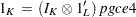
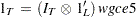
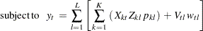
The optimization problem can be rewritten using set notation as follows
 |
 |
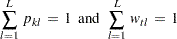 |
The subscript l denotes the support point (l=1, 2, ..., L), k denotes the parameter (k=1, 2, ..., K), and t denotes the observation (t=1, 2, ..., T).
The objective function is strictly convex; therefore, there is a unique global minimum for the problem (Golan, Judge, and Miller; 1996). The optimal estimated weights, p and w, and the prior supports, Z and V, can be used to form the point estimates of the unknown parameters,  , and the unknown errors, e, by using
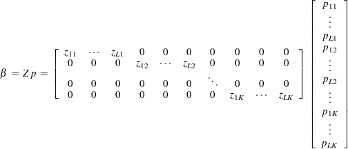 |
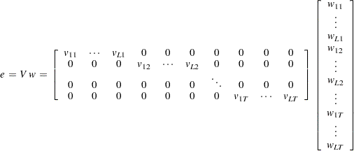 |
Computational Details
This constrained estimation problem can be solved either directly (primal) or by using the dual form. Either way, it is prudent to factor out one probability for each parameter and each observation as the sum of the other probabilities. This factoring reduces the computational complexity significantly. If the primal formalization is used and two support points are used for the parameters and the errors, the resulting GME problem is O . For the dual form, the problem is O
 . Therefore for large data sets, GME-M should be used instead of GME.
Note: This procedure is experimental.