The AUTOREG Procedure
- Overview
-
Getting Started

-
Syntax
-
Details
Missing Values Autoregressive Error Model Alternative Autocorrelation Correction Methods GARCH Models Heteroscedasticity Consistent Covariance Matrix Estimator Goodness-of-Fit Measures and Information Criteria Testing Predicted Values OUT= Data Set OUTEST= Data Set Printed Output ODS Table Names ODS Graphics
-
Examples
- References
| Regression with Autocorrelated Errors |
Ordinary regression analysis is based on several statistical assumptions. One key assumption is that the errors are independent of each other. However, with time series data, the ordinary regression residuals usually are correlated over time. It is not desirable to use ordinary regression analysis for time series data since the assumptions on which the classical linear regression model is based will usually be violated.
Violation of the independent errors assumption has three important consequences for ordinary regression. First, statistical tests of the significance of the parameters and the confidence limits for the predicted values are not correct. Second, the estimates of the regression coefficients are not as efficient as they would be if the autocorrelation were taken into account. Third, since the ordinary regression residuals are not independent, they contain information that can be used to improve the prediction of future values.
The AUTOREG procedure solves this problem by augmenting the regression model with an autoregressive model for the random error, thereby accounting for the autocorrelation of the errors. Instead of the usual regression model, the following autoregressive error model is used:


The notation  indicates that each
  is normally and independently distributed with mean 0 and variance
  .
.
By simultaneously estimating the regression coefficients  and the autoregressive error model parameters
  , the AUTOREG procedure corrects the regression estimates for autocorrelation. Thus, this kind of regression analysis is often called autoregressive error correction or serial correlation correction.
Example of Autocorrelated Data
A simulated time series is used to introduce the AUTOREG procedure. The following statements generate a simulated time series Y with second-order autocorrelation:
/* Regression with Autocorrelated Errors */
data a;
   ul = 0; ull = 0;
   do time = -10 to 36;
      u = + 1.3 * ul - .5 * ull + 2*rannor(12346);
      y = 10 + .5 * time + u;
      if time > 0 then output;
      ull = ul; ul = u;
   end;
run;
The series Y is a time trend plus a second-order autoregressive error. The model simulated is
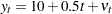


The following statements plot the simulated time series Y. A linear regression trend line is shown for reference.
title 'Autocorrelated Time Series';
proc sgplot data=a noautolegend;
   series x=time y=y / markers;
   reg x=time y=y/  lineattrs=(color=black);
run;
The plot of series Y and the regression line are shown in Figure 8.1.
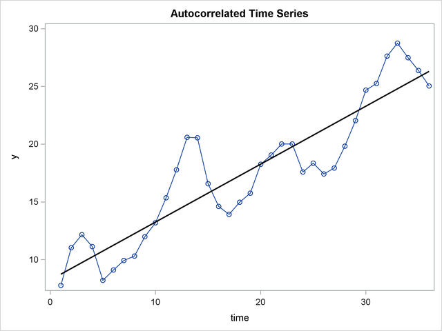
Note that when the series is above (or below) the OLS regression trend line, it tends to remain above (below) the trend for several periods. This pattern is an example of positive autocorrelation.
Time series regression usually involves independent variables other than a time trend. However, the simple time trend model is convenient for illustrating regression with autocorrelated errors, and the series Y shown in Figure 8.1 is used in the following introductory examples.
Ordinary Least Squares Regression
To use the AUTOREG procedure, specify the input data set in the PROC AUTOREG statement and specify the regression model in a MODEL statement. Specify the model by first naming the dependent variable and then listing the regressors after an equal sign, as is done in other SAS regression procedures. The following statements regress Y on TIME by using ordinary least squares:
proc autoreg data=a;
   model y = time;
run;
The AUTOREG procedure output is shown in Figure 8.2.
| Autocorrelated Time Series |
| Dependent Variable | y |
|---|
| Ordinary Least Squares Estimates | |||
|---|---|---|---|
| SSE | 214.953429 | DFE | 34 |
| MSE | 6.32216 | Root MSE | 2.51439 |
| SBC | 173.659101 | AIC | 170.492063 |
| MAE | 2.01903356 | AICC | 170.855699 |
| MAPE | 12.5270666 | HQC | 171.597444 |
| Durbin-Watson | 0.4752 | Regress R-Square | 0.8200 |
| Total R-Square | 0.8200 | ||
| Parameter Estimates | |||||
|---|---|---|---|---|---|
| Variable | DF | Estimate | Standard Error | t Value | Approx Pr > |t| |
| Intercept | 1 | 8.2308 | 0.8559 | 9.62 | <.0001 |
| time | 1 | 0.5021 | 0.0403 | 12.45 | <.0001 |
The output first shows statistics for the model residuals. The model root mean square error (Root MSE) is 2.51, and the model  is 0.82. Notice that two statistics are shown, one for the regression model (Reg Rsq) and one for the full model (Total Rsq) that includes the autoregressive error process, if any. In this case, an autoregressive error model is not used, so the two statistics are the same.
Other statistics shown are the sum of square errors (SSE), mean square error (MSE), mean absolute error (MAE), mean absolute percentage error (MAPE), error degrees of freedom (DFE, the number of observations minus the number of parameters), the information criteria SBC, HQC, AIC, and AICC, and the Durbin-Watson statistic. (Durbin-Watson statistics, MAE, MAPE, SBC, HQC, AIC, and AICC are discussed in the section Goodness-of-Fit Measures and Information Criteria.)
The output then shows a table of regression coefficients, with standard errors and t tests. The estimated model is
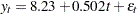
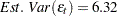
The OLS parameter estimates are reasonably close to the true values, but the estimated error variance, 6.32, is much larger than the true value, 4.
Autoregressive Error Model
The following statements regress Y on TIME with the errors assumed to follow a second-order autoregressive process. The order of the autoregressive model is specified by the NLAG=2 option. The Yule-Walker estimation method is used by default. The example uses the METHOD=ML option to specify the exact maximum likelihood method instead.
proc autoreg data=a;
   model y = time / nlag=2 method=ml;
run;
The first part of the results is shown in Figure 8.3. The initial OLS results are produced first, followed by estimates of the autocorrelations computed from the OLS residuals. The autocorrelations are also displayed graphically.
| Autocorrelated Time Series |
| Dependent Variable | y |
|---|
| Ordinary Least Squares Estimates | |||
|---|---|---|---|
| SSE | 214.953429 | DFE | 34 |
| MSE | 6.32216 | Root MSE | 2.51439 |
| SBC | 173.659101 | AIC | 170.492063 |
| MAE | 2.01903356 | AICC | 170.855699 |
| MAPE | 12.5270666 | HQC | 171.597444 |
| Durbin-Watson | 0.4752 | Regress R-Square | 0.8200 |
| Total R-Square | 0.8200 | ||
| Parameter Estimates | |||||
|---|---|---|---|---|---|
| Variable | DF | Estimate | Standard Error | t Value | Approx Pr > |t| |
| Intercept | 1 | 8.2308 | 0.8559 | 9.62 | <.0001 |
| time | 1 | 0.5021 | 0.0403 | 12.45 | <.0001 |
| Estimates of Autocorrelations | |||
|---|---|---|---|
| Lag | Covariance | Correlation | -1 9 8 7 6 5 4 3 2 1 0 1 2 3 4 5 6 7 8 9 1 |
| 0 | 5.9709 | 1.000000 | | |********************| |
| 1 | 4.5169 | 0.756485 | | |*************** | |
| 2 | 2.0241 | 0.338995 | | |******* | |
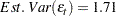
| Preliminary MSE | 1.7943 |
|---|
The maximum likelihood estimates are shown in Figure 8.4. Figure 8.4 also shows the preliminary Yule-Walker estimates used as starting values for the iterative computation of the maximum likelihood estimates.
| Estimates of Autoregressive Parameters | |||
|---|---|---|---|
| Lag | Coefficient | Standard Error | t Value |
| 1 | -1.169057 | 0.148172 | -7.89 |
| 2 | 0.545379 | 0.148172 | 3.68 |
| Algorithm converged. |
| Maximum Likelihood Estimates | |||
|---|---|---|---|
| SSE | 54.7493022 | DFE | 32 |
| MSE | 1.71092 | Root MSE | 1.30802 |
| SBC | 133.476508 | AIC | 127.142432 |
| MAE | 0.98307236 | AICC | 128.432755 |
| MAPE | 6.45517689 | HQC | 129.353194 |
| Log Likelihood | -59.571216 | Regress R-Square | 0.7280 |
| Durbin-Watson | 2.2761 | Total R-Square | 0.9542 |
| Observations | 36 | ||
| Parameter Estimates | |||||
|---|---|---|---|---|---|
| Variable | DF | Estimate | Standard Error | t Value | Approx Pr > |t| |
| Intercept | 1 | 7.8833 | 1.1693 | 6.74 | <.0001 |
| time | 1 | 0.5096 | 0.0551 | 9.25 | <.0001 |
| AR1 | 1 | -1.2464 | 0.1385 | -9.00 | <.0001 |
| AR2 | 1 | 0.6283 | 0.1366 | 4.60 | <.0001 |
| Autoregressive parameters assumed given | |||||
|---|---|---|---|---|---|
| Variable | DF | Estimate | Standard Error | t Value | Approx Pr > |t| |
| Intercept | 1 | 7.8833 | 1.1678 | 6.75 | <.0001 |
| time | 1 | 0.5096 | 0.0551 | 9.26 | <.0001 |
The diagnostic statistics and parameter estimates tables in Figure 8.4 have the same form as in the OLS output, but the values shown are for the autoregressive error model. The MSE for the autoregressive model is 1.71, which is much smaller than the true value of 4. In small samples, the autoregressive error model tends to underestimate , while the OLS MSE overestimates .
Notice that the total statistic computed from the autoregressive model residuals is 0.954, reflecting the improved fit from the use of past residuals to help predict the next Y value. The Reg Rsq value 0.728 is the statistic for a regression of transformed variables adjusted for the estimated autocorrelation. (This is not the for the estimated trend line. For details, see the section Goodness-of-Fit Measures and Information Criteria later in this chapter.)
The parameter estimates table shows the ML estimates of the regression coefficients and includes two additional rows for the estimates of the autoregressive parameters, labeled AR(1) and AR(2).
The estimated model is
 |
 |
 |
Note that the signs of the autoregressive parameters shown in this equation for  are the reverse of the estimates shown in the AUTOREG procedure output. Figure 8.4 also shows the estimates of the regression coefficients with the standard errors recomputed on the assumption that the autoregressive parameter estimates equal the true values.
Predicted Values and Residuals
The AUTOREG procedure can produce two kinds of predicted values and corresponding residuals and confidence limits. The first kind of predicted value is obtained from only the structural part of the model,  . This is an estimate of the unconditional mean of the response variable at time t. For the time trend model, these predicted values trace the estimated trend. The second kind of predicted value includes both the structural part of the model and the predicted values of the autoregressive error process. The full model (conditional) predictions are used to forecast future values.
Use the OUTPUT statement to store predicted values and residuals in a SAS data set and to output other values such as confidence limits and variance estimates. The P= option specifies an output variable to contain the full model predicted values. The PM= option names an output variable for the predicted mean. The R= and RM= options specify output variables for the corresponding residuals, computed as the actual value minus the predicted value.
The following statements store both kinds of predicted values in the output data set. (The printed output is the same as previously shown in Figure 8.3 and Figure 8.4.)
proc autoreg data=a;
   model y = time / nlag=2 method=ml;
   output out=p p=yhat pm=trendhat;
run;
The following statements plot the predicted values from the regression trend line and from the full model together with the actual values:
title 'Predictions for Autocorrelation Model';
proc sgplot data=p;
   scatter x=time y=y / markerattrs=(color=blue);
   series x=time y=yhat / lineattrs=(color=blue);
   series x=time y=trendhat / lineattrs=(color=black);
run;
The plot of predicted values is shown in Figure 8.5.
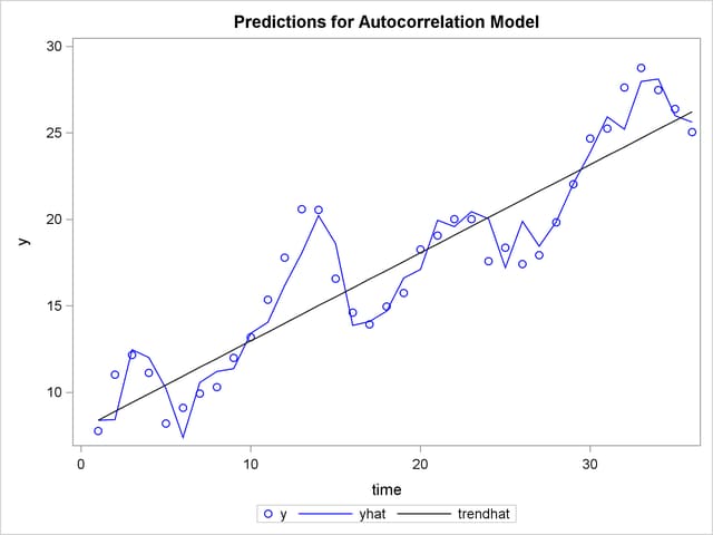
In Figure 8.5 the straight line is the autocorrelation corrected regression line, traced out by the structural predicted values TRENDHAT. The jagged line traces the full model prediction values. The actual values are marked by asterisks. This plot graphically illustrates the improvement in fit provided by the autoregressive error process for highly autocorrelated data.