| The MODEL Procedure |
Example 18.13 Switching Regression Example
Take the usual linear regression problem
 |
where Y denotes the n column vector of the dependent variable,  denotes the (n
  k ) matrix of independent variables,
  denotes the k column vector of coefficients to be estimated, n denotes the number of observations (i =1, 2, ..., n ), and k denotes the number of independent variables.
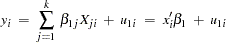
You can take this basic equation and split it into two regimes, where the ith observation on y is generated by one regime or the other:
 |
|||
 |
where  and
and  are the ith and jth observations, respectively, on
  . The errors,
  and
and  , are assumed to be distributed normally and independently with mean zero and constant variance. The variance for the first regime is
  , and the variance for the second regime is
  . If
. If  and
and  , the regression system given previously is thought to be switching between the two regimes.
The problem is to estimate  ,
,  ,
,  , and
, and  without knowing a priori which of the n values of the dependent variable, y, was generated by which regime. If it is known a priori which observations belong to which regime, a simple Chow test can be used to test
  and
and  .
.
Using Goldfeld and Quandt’s D-method for switching regression, you can solve this problem. Assume that observations exist on some exogenous variables  , where z determines whether the ith observation is generated from one equation or the other. The equations are given as follows:
 |
 |
 |
|||
 |
|
 |
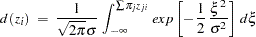
where  are unknown coefficients to be estimated. Define
  as a continuous approximation to a step function. Replacing the unit step function with a continuous approximation by using the cumulative normal integral enables a more practical method that produces consistent estimates.
 |
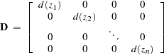
 is the n dimensional diagonal matrix consisting of :
 |
The parameters to estimate are now the k ’s, the k ’s, , , p  ’s, and the
  introduced in the
  equation. The
  can be considered as given a priori, or it can be estimated, in which case, the estimated magnitude provides an estimate of the success in discriminating between the two regimes (Goldfeld and Quandt 1976). Given the preceding equations, the model can be written as:
 |
where  , and W is a vector of unobservable and heteroscedastic error terms. The covariance matrix of W is denoted by
  , where
 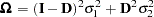 . The maximum likelihood parameter estimates maximize the following log-likelihood function.
 |
|
 |
|||
 |
|
 |
As an example, you now can use this switching regression likelihood to develop a model of housing starts as a function of changes in mortgage interest rates. The data for this example are from the U.S. Census Bureau and cover the period from January 1973 to March 1999. The hypothesis is that there are different coefficients on your model based on whether the interest rates are going up or down.
So the model for  is
is
 |
where  is the mortgage interest rate at time
  and
and  is a scale parameter to be estimated.
The regression model is
 |
 |
 |
|||
 |
|
 |
where  is the number of housing starts at month and
  is a dummy variable that indicates that the current month is one of December, January, or February.
This model is written by using the following SAS statements:
   title1 'Switching Regression Example';

   proc model data=switch;
      parms sig1=10 sig2=10 int1 b11 b13 int2 b21 b23 p;
      bounds 0.0001 < sig1 sig2;

      decjanfeb = ( month(date) = 12 | month(date) <= 2 );

      a = p*dif(rate);       /* Upper bound of integral */
      d = probnorm(a);       /* Normal CDF as an approx of switch */

                             /* Regime 1 */
      y1 = int1 + zlag(starts)*b11 + decjanfeb *b13 ;
                             /* Regime 2 */
      y2 = int2 + zlag(starts)*b21 + decjanfeb *b23 ;
                             /* Composite regression equation */
      starts  = (1 - d)*y1 +  d*y2;

                            /* Resulting log-likelihood function */
      logL = (1/2)*( (log(2*3.1415)) +
           log( (sig1**2)*((1-d)**2)+(sig2**2)*(d**2) )
          + (resid.starts*( 1/( (sig1**2)*((1-d)**2)+
           (sig2**2)*(d**2) ) )*resid.starts) ) ;

      errormodel starts ~ general(logL);

      fit starts / method=marquardt converge=1.0e-5;

        /* Test for significant differences in the parms */
      test int1 = int2 ,/ lm;
      test b11 = b21 ,/ lm;
      test b13 = b23 ,/ lm;
      test sig1 = sig2 ,/ lm;

   run;
Four TEST statements are added to test the hypothesis that the parameters are the same in both regimes. The parameter estimates and ANOVA table from this run are shown in Output 18.13.1.
| Nonlinear Liklhood Summary of Residual Errors | ||||||||
|---|---|---|---|---|---|---|---|---|
| Equation | DF Model | DF Error | SSE | MSE | Root MSE | R-Square | Adj R-Sq | Label |
| starts | 9 | 304 | 85878.0 | 282.5 | 16.8075 | 0.7806 | 0.7748 | Housing Starts |
| Nonlinear Liklhood Parameter Estimates | ||||
|---|---|---|---|---|
| Parameter | Estimate | Approx Std Err | t Value | Approx Pr > |t| |
| sig1 | 15.47484 | 0.9476 | 16.33 | <.0001 |
| sig2 | 19.77808 | 1.2710 | 15.56 | <.0001 |
| int1 | 32.82221 | 5.9083 | 5.56 | <.0001 |
| b11 | 0.73952 | 0.0444 | 16.64 | <.0001 |
| b13 | -15.4556 | 3.1912 | -4.84 | <.0001 |
| int2 | 42.73348 | 6.8159 | 6.27 | <.0001 |
| b21 | 0.734117 | 0.0478 | 15.37 | <.0001 |
| b23 | -22.5184 | 4.2985 | -5.24 | <.0001 |
| p | 25.94712 | 8.5205 | 3.05 | 0.0025 |
The test results shown in Output 18.13.2 suggest that the variance of the housing starts, SIG1 and SIG2, are significantly different in the two regimes. The tests also show a significant difference in the AR term on the housing starts.
Copyright © 2008 by SAS Institute Inc., Cary, NC, USA. All rights reserved.