PROC MODEL: Circuit Estimation :: SAS/ETS(R) 9.2 User's Guide

The MODEL Procedure

Example 18.9 Circuit Estimation

Consider the nonlinear circuit shown in Figure 18.92.

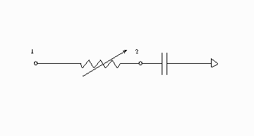
Figure 18.92 Nonlinear Resistor Capacitor Circuit

$\includegraphics{png/modcirc}$

The theory of electric circuits is governed by Kirchhoff’s laws: the sum of the currents flowing to a node is zero, and the net voltage drop around a closed loop is zero. In addition to Kirchhoff’s laws, there are relationships between the current I through each element and the voltage drop V across the elements. For the circuit in Figure 18.92, the relationships are

$\text{[math]}$

for the capacitor and

$\text{[math]}$

for the nonlinear resistor. The following differential equation describes the current at node 2 as a function of time and voltage for this circuit:

$\text{[math]}$

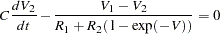This equation can be written in the form

$\text{[math]}$

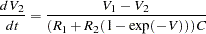Consider the following data.

   data circ;
      input v2 v1 time@@;
   datalines;
   -0.00007 0.0 0.0000000001 0.00912 0.5 0.0000000002
    0.03091 1.0 0.0000000003 0.06419 1.5 0.0000000004
    0.11019 2.0 0.0000000005 0.16398 2.5 0.0000000006
    0.23048 3.0 0.0000000007 0.30529 3.5 0.0000000008
    0.39394 4.0 0.0000000009 0.49121 4.5 0.0000000010
    0.59476 5.0 0.0000000011 0.70285 5.0 0.0000000012
    0.81315 5.0 0.0000000013 0.90929 5.0 0.0000000014
    1.01412 5.0 0.0000000015 1.11386 5.0 0.0000000016
    1.21106 5.0 0.0000000017 1.30237 5.0 0.0000000018
    1.40461 5.0 0.0000000019 1.48624 5.0 0.0000000020
    1.57894 5.0 0.0000000021 1.66471 5.0 0.0000000022
   ;

You can estimate the parameters in the preceding equation by using the following SAS statements:

   title1 'Circuit Model Estimation Example';
   
   proc model data=circ mintimestep=1.0e-23;
      parm R2 2000  R1 4000 C 5.0e-13;
      dert.v2 = (v1-v2)/((r1 + r2*(1-exp( -(v1-v2)))) * C);
      fit v2;
   run;

The results of the estimation are shown in Output 18.9.1.

Output 18.9.1 Circuit Estimation

Circuit Model Estimation Example

The MODEL Procedure

Nonlinear OLS Parameter Estimates
Parameter	Estimate	Approx Std Err	t Value	Approx Pr > \|t\|
R2	3002.465	1517.1	<------	Biased
R1	4984.848	1466.8	<------	Biased
C	5E-13	0	<------	Biased

Note:

The model was singular. Some estimates are marked 'Biased'.

In this case, the model equation is such that there is linear dependency that causes biased results and inflated variances. The Jacobian matrix is singular or nearly singular, but eliminating one of the parameters is not a solution in this case.

Top of Page