| The MODEL Procedure |
Example 18.7 Spring and Damper Continuous System
This model simulates the mechanical behavior of a spring and damper system shown in Figure 18.92.
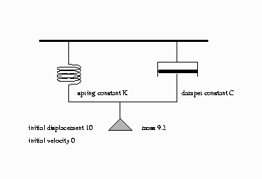
A mass is hung from a spring with spring constant K. The motion is slowed by a damper with damper constant C. The damping force is proportional to the velocity, while the spring force is proportional to the displacement.
This is actually a continuous system; however, the behavior can be approximated by a discrete time model. We approximate the differential equation
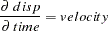 |
with the difference equation
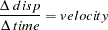 |
This is rewritten as
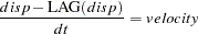 |
where dt is the time step used. In PROC MODEL, this is expressed with the program statement
disp = lag(disp) + vel * dt;
or
dert.disp = vel;
The first statement is simply a computing formula for Euler’s approximation for the integral
 |
If the time step is small enough with respect to the changes in the system, the approximation is good. Although PROC MODEL does not have the variable step-size and error-monitoring features of simulators designed for continuous systems, the procedure is a good tool to use for less challenging continuous models.
The second form instructs the MODEL procedure to do the integration for you.
This model is unusual because there are no exogenous variables, and endogenous data are not needed. Although you still need a SAS data set to count the simulation periods, no actual data are brought in.
Since the variables DISP and VEL are lagged, initial values specified in the VAR statement determine the starting state of the system. The mass, time step, spring constant, and damper constant are declared and initialized by a CONTROL statement as shown in the following statements:
   title1 'Simulation of Spring-Mass-Damper System';

   /*- Data to drive the simulation time periods ---*/
   data one;
      do n=1 to 100;
         output;
      end;
   run;

   proc model data=one outmodel=spring;
      var      force -200  disp  10  vel  0  accel -20  time 0;
      control  mass   9.2  c    1.5  dt  .1  k      20;
      force = -k * disp -c * vel;
      disp  = lag(disp) + vel * dt;
      vel   = lag(vel) + accel * dt;
      accel = force / mass;
      time  = lag(time) + dt;
   run;
The displacement scale is zeroed at the point where the force of gravity is offset, so the acceleration of the gravity constant is omitted from the force equation. The control variable C and K represent the damper and the spring constants respectively.
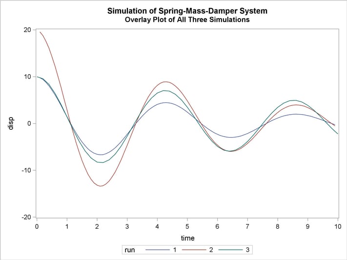
The model is simulated three times, and the simulation results are written to output data sets. The first run uses the original initial conditions specified in the VAR statement. In the second run, the initial displacement is doubled; the results show that the period of the motion is unaffected by the amplitude. In the third run, the DERT. syntax is used to do the integration. Notice that the path of the displacement is close to the old path, indicating that the original time step is short enough to yield an accurate solution. These simulations are performed by the following statements:
   proc model data=one model=spring;
      title2 "Simulation of the model for the base case";
      control run '1';
      solve / out=a;
   run;

      title2 "Simulation of the model with twice the initial displacement";
      control run '2';
      var disp 20;
      solve / out=b;
   run;
   data two;
      do time = 0 to 10 by .2; output;end;
   run;

   title2 "Simulation of the model using the dert. syntax";
   proc model data=two;
      var      force -200  disp  10  vel  0  accel -20  time 0;
      control  mass   9.2  c    1.5  dt  .1  k      20;
      control run '3' ;
      force = -k * disp -c * vel;
      dert.disp  = vel ;
      dert.vel   = accel;
      accel = force / mass;
      solve / out=c;
      id time ;
   run;
The output SAS data sets that contain the solution results are merged and the displacement time paths for the three simulations are plotted. The three runs are identified on the plot as 1, 2, and 3. The following statements produce Output 18.7.1 through Output 18.7.5.
   data p;
      set a b c;
   run;

   title2 'Overlay Plot of All Three Simulations';
   proc sgplot data=p;
      series x=time y=disp / group=run lineattrs=(pattern=1);
      xaxis values=(0 to 10 by 1);
      yaxis values=(-20 to 20 by 10);
   run;
| Model Summary | |
|---|---|
| Model Variables | 5 |
| Control Variables | 5 |
| Equations | 5 |
| Number of Statements | 6 |
| Program Lag Length | 1 |
| Data Set Options | |
|---|---|
| DATA= | ONE |
| OUT= | A |
| Solution Summary | |
|---|---|
| Variables Solved | 5 |
| Simulation Lag Length | 1 |
| Solution Method | NEWTON |
| CONVERGE= | 1E-8 |
| Maximum CC | 8.68E-15 |
| Maximum Iterations | 1 |
| Total Iterations | 99 |
| Average Iterations | 1 |
| Data Set Options | |
|---|---|
| DATA= | ONE |
| OUT= | B |
| Solution Summary | |
|---|---|
| Variables Solved | 5 |
| Simulation Lag Length | 1 |
| Solution Method | NEWTON |
| CONVERGE= | 1E-8 |
| Maximum CC | 2.64E-14 |
| Maximum Iterations | 1 |
| Total Iterations | 99 |
| Average Iterations | 1 |
| Data Set Options | |
|---|---|
| DATA= | TWO |
| OUT= | C |
Copyright © 2008 by SAS Institute Inc., Cary, NC, USA. All rights reserved.