| The MODEL Procedure |
| Nonlinear Regression Analysis |
One of the most important uses of PROC MODEL is to estimate unknown parameters in a nonlinear model. A simple nonlinear model has the form:
 |
where x is a vector of exogenous variables. To estimate unknown parameters by using PROC MODEL, do the following:
Use the DATA= option in a PROC MODEL statement to specify the input SAS data set that contains
 and
and  , the observed values of the variables.
 Write the equation for the model by using SAS programming statements, including all parameters and arithmetic operators but leaving off the unobserved error component,
 .
. Use a FIT statement to fit the model equation to the input data to determine the unknown parameters,
 .
.
An Example
The SASHELP library contains the data set CITIMON, which contains the variable LHUR, the monthly unemployment figures, and the variable IP, the monthly industrial production index. You suspect that the unemployment rates are inversely proportional to the industrial production index. Assume that these variables are related by the following nonlinear equation:
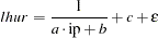 |
In this equation a, b, and c are unknown coefficients and  is an unobserved random error.
The following statements illustrate how to use PROC MODEL to estimate values for a, b, and c from the data in SASHELP.CITIMON.
   proc model data=sashelp.citimon;
      lhur = 1/(a * ip + b) + c;
      fit lhur;
   run;
Notice that the model equation is written as a SAS assignment statement. The variable LHUR is assumed to be the dependent variable because it is named in the FIT statement and is on the left-hand side of the assignment.
PROC MODEL determines that LHUR and IP are observed variables because they are in the input data set. A, B, and C are treated as unknown parameters to be estimated from the data because they are not in the input data set. If the data set contained a variable named A, B, or C, you would need to explicitly declare the parameters with a PARMS statement.
In response to the FIT statement, PROC MODEL estimates values for A, B, and C by using nonlinear least squares and prints the results. The first part of the output is a "Model Summary" table, shown in Figure 18.1.
| Model Summary | |
|---|---|
| Model Variables | 1 |
| Parameters | 3 |
| Equations | 1 |
| Number of Statements | 1 |
This table details the size of the model, including the number of programming statements that define the model, and lists the dependent variables (LHUR in this case), the unknown parameters (A, B, and C), and the model equations. In this case the equation is named for the dependent variable, LHUR.
PROC MODEL then prints a summary of the estimation problem, as shown in Figure 18.2.
The notation used in the summary of the estimation problem indicates that LHUR is a function of A, B, and C, which are to be estimated by fitting the function to the data. If the partial derivative of the equation with respect to a parameter is a simple variable or constant, the derivative is shown in parentheses after the parameter name. In this case, the derivative with respect to the intercept C is 1. The derivatives with respect to A and B are complex expressions and so are not shown.
Next, PROC MODEL prints an estimation summary as shown in Figure 18.3.
| Data Set Options | |
|---|---|
| DATA= | SASHELP.CITIMON |
| Final Convergence Criteria | |
|---|---|
| R | 0.000737 |
| PPC(b) | 0.003943 |
| RPC(b) | 0.00968 |
| Object | 4.784E-6 |
| Trace(S) | 0.533325 |
| Objective Value | 0.522214 |
The estimation summary provides information on the iterative process used to compute the estimates. The heading "OLS Estimation Summary" indicates that the nonlinear ordinary least squares (OLS) estimation method is used. This table indicates that all three parameters were estimated successfully by using 144 nonmissing observations from the data set SASHELP.CITIMON. Calculating the estimates required 10 iterations of the GAUSS method. Various measures of how well the iterative process converged are also shown. For example, the "RPC(B)" value 0.00968 means that on the final iteration the largest relative change in any estimate was for parameter B, which changed by 0.968 percent. See the section Convergence Criteria for details.
PROC MODEL then prints the estimation results. The first part of this table is the summary of residual errors, shown in Figure 18.4.
| Nonlinear OLS Summary of Residual Errors | ||||||||
|---|---|---|---|---|---|---|---|---|
| Equation | DF Model | DF Error | SSE | MSE | Root MSE | R-Square | Adj R-Sq | Label |
| LHUR | 3 | 141 | 75.1989 | 0.5333 | 0.7303 | 0.7472 | 0.7436 | UNEMPLOYMENT RATE: ALL WORKERS, 16 YEARS |
This table lists the sum of squared errors (SSE), the mean squared error (MSE), the root mean squared error (root MSE), and the R and adjusted R statistics. The R value of 0.7472 means that the estimated model explains approximately 75 percent more of the variability in LHUR than a mean model explains.
Following the summary of residual errors is the parameter estimates table, shown in Figure 18.5.
Because the model is nonlinear, the standard error of the estimate, the t value, and its significance level are only approximate. These values are computed using asymptotic formulas that are correct for large sample sizes but only approximately correct for smaller samples. Thus, you should use caution in interpreting these statistics for nonlinear models, especially for small sample sizes. For linear models, these results are exact and are the same as standard linear regression.
The last part of the output produced by the FIT statement is shown in Figure 18.6.
This table lists the objective value for the estimation of the nonlinear system. Since there is only a single equation in this case, the objective value is the same as the residual MSE for LHUR except that the objective value does not include a degrees-of-freedom correction. This can be seen in the fact that "Objective*N" equals the residual SSE, 75.1989. N is 144, the number of observations used.
Convergence and Starting Values
Computing parameter estimates for nonlinear equations requires an iterative process. Starting with an initial guess for the parameter values, PROC MODEL tries different parameter values until the objective function of the estimation method is minimized. (The objective function of the estimation method is sometimes called the fitting function.) This process does not always succeed, and whether it does succeed depends greatly on the starting values used. By default, PROC MODEL uses the starting value 0.0001 for all parameters.
Consequently, in order to use PROC MODEL to achieve convergence of parameter estimates, you need to know two things: how to recognize convergence failure by interpreting diagnostic output, and how to specify reasonable starting values. The MODEL procedure includes alternate iterative techniques and grid search capabilities to aid in finding estimates. See the section Troubleshooting Convergence Problems for more details.
Copyright © 2008 by SAS Institute Inc., Cary, NC, USA. All rights reserved.