| The MODEL Procedure |
| Troubleshooting Convergence Problems |
As with any nonlinear estimation routine, there is no guarantee that the estimation will be successful for a given model and data. If the equations are linear with respect to the parameters, the parameter estimates always converge in one iteration. The methods that iterate the S matrix must iterate further for the S matrix to converge. Nonlinear models might not necessarily converge.
Convergence can be expected only with fully identified parameters, adequate data, and starting values sufficiently close to solution estimates.
Convergence and the rate of convergence might depend primarily on the choice of starting values for the estimates. This does not mean that a great deal of effort should be invested in choosing starting values. First, try the default values. If the estimation fails with these starting values, examine the model and data and rerun the estimation using reasonable starting values. It is usually not necessary that the starting values be very good, just that they not be very bad; choose values that seem plausible for the model and data.
An Example of Requiring Starting Values
Suppose you want to regress a variable Y on a variable X, assuming that the variables are related by the following nonlinear equation:
 |
In this equation, Y is linearly related to a power transformation of X. The unknown parameters are a, b, and c.  is an unobserved random error. The following SAS statements generate simulated data. In this simulation,
  ,
,  , and the use of the SQRT function corresponds to
  .
.
   data test;
     do i = 1 to 20;
        x = 5 * ranuni(1234);
        y = 10 + 2 * sqrt(x) + .5 * rannor(2345);
        output;
        end;
   run;
The following statements specify the model and give descriptive labels to the model parameters. Then the FIT statement attempts to estimate a, b, and c by using the default starting value 0.0001.
   proc model data=test;
      y = a + b * x ** c;
      label a = "Intercept"
            b = "Coefficient of Transformed X"
            c = "Power Transformation Parameter";
      fit y;
   run;
PROC MODEL prints model summary and estimation problem summary reports and then prints the output shown in Figure 18.24.
| ERROR: The parameter estimates failed to converge for OLS after 100 iterations using CONVERGE=0.001 as the convergence criteria. |
By using the default starting values, PROC MODEL is unable to take even the first step in iterating to the solution. The change in the parameters that the Gauss-Newton method computes is very extreme and makes the objective values worse instead of better. Even when this step is shortened by a factor of a million, the objective function is still worse, and PROC MODEL is unable to estimate the model parameters.
The problem is caused by the starting value of C. Using the default starting value C=0.0001, the first iteration attempts to compute better values of A and B by what is, in effect, a linear regression of Y on the 10,000th root of X, which is almost the same as the constant 1. Thus the matrix that is inverted to compute the changes is nearly singular and affects the accuracy of the computed parameter changes.
This is also illustrated by the next part of the output, which displays collinearity diagnostics for the crossproducts matrix of the partial derivatives with respect to the parameters, shown in Figure 18.25.
This output shows that the matrix is singular and that the partials of A, B, and C with respect to the residual are collinear at the point  in the parameter space. See the section Linear Dependencies for a full explanation of the collinearity diagnostics.
The MODEL procedure next prints the note shown in Figure 18.26, which suggests that you try different starting values.
| Note: | The parameter estimation is abandoned. Check your model and data. If the model is correct and the input data are appropriate, try rerunning the parameter estimation using different starting values for the parameter estimates. PROC MODEL continues as if the parameter estimates had converged. |
PROC MODEL then produces the usual printout of results for the nonconverged parameter values. The estimation summary is shown in Figure 18.27. The heading includes the reminder "(Not Converged)".
| Data Set Options | |
|---|---|
| DATA= | TEST |
| Minimization Summary | |
|---|---|
| Parameters Estimated | 3 |
| Method | Gauss |
| Iterations | 100 |
| Subiterations | 239 |
| Average Subiterations | 2.39 |
| Final Convergence Criteria | |
|---|---|
| R | 0.962666 |
| PPC(b) | 548.2193 |
| RPC(b) | 540.3066 |
| Object | 2.654E-6 |
| Trace(S) | 4.667946 |
| Objective Value | 3.967754 |
The nonconverged estimation results are shown in Figure 18.28.
| Nonlinear OLS Summary of Residual Errors (Not Converged) |
|||||||
|---|---|---|---|---|---|---|---|
| Equation | DF Model | DF Error | SSE | MSE | Root MSE | R-Square | Adj R-Sq |
| y | 3 | 17 | 79.3551 | 4.6679 | 2.1605 | -1.6812 | -1.9966 |
| Nonlinear OLS Parameter Estimates (Not Converged) | |||||
|---|---|---|---|---|---|
| Parameter | Estimate | Approx Std Err | t Value | Approx Pr > |t| |
Label |
| a | 137.3822 | 263349 | 0.00 | 0.9996 | Intercept |
| b | -126.533 | 263349 | -0.00 | 0.9996 | Coefficient of Transformed X |
| c | -0.00213 | 4.4373 | -0.00 | 0.9996 | Power Transformation Parameter |
 statistic is negative. An < 0 results when the residual mean squared error for the model is larger than the variance of the dependent variable. Negative R
 statistics might be produced when either the parameter estimates fail to converge correctly, as in this case, or when the correctly estimated model fits the data very poorly.
Controlling Starting Values
To fit the preceding model you must specify a better starting value for C. Avoid starting values of C that are either very large or close to 0. For starting values of A and B, you can specify values, use the default, or have PROC MODEL fit starting values for them conditional on the starting value for C.
Starting values are specified with the START= option of the FIT statement or in a PARMS statement. In PROC MODEL, you have several options to specify starting values for the parameters to be estimated. When more than one option is specified, the options are implemented in the following order of precedence (from highest to lowest): the START= option, the PARMS statement initialization value, the ESTDATA= option, and the PARMSDATA= option. When no starting values for the parameter estimates are specified with BY group processing, the default start value 0.0001 is used for each by group. Again, when no starting values are specified, and a model with a FIT statement is stored by the OUTMODEL=outmodel-filename option in a previous step, the outmodel-filename can be invoked in a subsequent PROC MODEL step by using the MODEL=outmodel-filename option with multiple estimation methods in the second step. In such a case, the parameter estimates from the outmodel-filename are used directly as starting values for OLS, and OLS results from the second step provide starting values for the subsequent estimation method such as 2SLS or SUR, provided that NOOLS is not specified.
For example, the following statements estimate the model parameters by using the starting values A=0.0001, B=0.0001, and C=5.
   proc model data=test;
      y = a + b * x ** c;
      label a = "Intercept"
            b = "Coefficient of Transformed X"
            c = "Power Transformation Parameter";
      fit y start=(c=5);
   run;
Using these starting values, the estimates converge in 16 iterations. The results are shown in Figure 18.29. Note that since the START= option explicitly declares parameters, the parameter C is placed first in the table.
| Nonlinear OLS Summary of Residual Errors | |||||||
|---|---|---|---|---|---|---|---|
| Equation | DF Model | DF Error | SSE | MSE | Root MSE | R-Square | Adj R-Sq |
| y | 3 | 17 | 5.7359 | 0.3374 | 0.5809 | 0.8062 | 0.7834 |
| Nonlinear OLS Parameter Estimates | |||||
|---|---|---|---|---|---|
| Parameter | Estimate | Approx Std Err | t Value | Approx Pr > |t| |
Label |
| c | 0.327079 | 0.2892 | 1.13 | 0.2738 | Power Transformation Parameter |
| a | 8.384311 | 3.3775 | 2.48 | 0.0238 | Intercept |
| b | 3.505391 | 3.4858 | 1.01 | 0.3287 | Coefficient of Transformed X |
Using the STARTITER Option
PROC MODEL can compute starting values for some parameters conditional on starting values you specify for the other parameters. You supply starting values for some parameters and specify the STARTITER option on the FIT statement.
For example, the following statements set C to 1 and compute starting values for A and B by estimating these parameters conditional on the fixed value of C. With C=1, this is equivalent to computing A and B by linear regression on X. A PARMS statement is used to declare the parameters in alphabetical order. The ITPRINT option is used to print the parameter values at each iteration.
   proc model data=test;
      parms a b c;
      y = a + b * x ** c;
      label a = "Intercept"
            b = "Coefficient of Transformed X"
            c = "Power Transformation Parameter";
      fit y start=(c=1) / startiter itprint;
   run;
With better starting values, the estimates converge in only eight iterations. Counting the iteration required to compute the starting values for A and B, this is seven fewer than the 16 iterations required without the STARTITER option. The iteration history listing is shown in Figure 18.30.
| Iteration | N Obs | R | Objective | N Subit | a | b | c | |
|---|---|---|---|---|---|---|---|---|
| GRID | 0 | 20 | 0.9989 | 162.9 | 0 | 0.00010 | 0.00010 | 1.00000 |
| GRID | 1 | 20 | 0.0000 | 0.3464 | 0 | 10.96530 | 0.77007 | 1.00000 |
| Iteration | N Obs | R | Objective | N Subit | a | b | c | |
|---|---|---|---|---|---|---|---|---|
| OLS | 0 | 20 | 0.3873 | 0.3464 | 0 | 10.96530 | 0.77007 | 1.00000 |
| OLS | 1 | 20 | 0.3339 | 0.3282 | 2 | 10.75993 | 0.99433 | 0.83096 |
| OLS | 2 | 20 | 0.3244 | 0.3233 | 1 | 10.46894 | 1.31205 | 0.66810 |
| OLS | 3 | 20 | 0.3151 | 0.3197 | 1 | 10.11707 | 1.69149 | 0.54626 |
| OLS | 4 | 20 | 0.2764 | 0.3110 | 1 | 9.74691 | 2.08492 | 0.46615 |
| OLS | 5 | 20 | 0.2379 | 0.3040 | 0 | 9.06175 | 2.80546 | 0.36575 |
| OLS | 6 | 20 | 0.0612 | 0.2879 | 0 | 8.51825 | 3.36746 | 0.33201 |
| OLS | 7 | 20 | 0.0022 | 0.2868 | 0 | 8.39485 | 3.49449 | 0.32776 |
| OLS | 8 | 20 | 0.0001 | 0.2868 | 0 | 8.38467 | 3.50502 | 0.32711 |
The results produced in this case are almost the same as the results shown in Figure 18.29, except that the PARMS statement causes the parameter estimates table to be ordered A, B, C instead of C, A, B. They are not exactly the same because the different starting values caused the iterations to converge at a slightly different place. This effect is controlled by changing the convergence criterion with the CONVERGE= option.
By default, the STARTITER option performs one iteration to find starting values for the parameters that are not given values. In this case, the model is linear in A and B, so only one iteration is needed. If A or B were nonlinear, you could specify more than one "starting values" iteration by specifying a number for the STARTITER= option.
Finding Starting Values by Grid Search
PROC MODEL can try various combinations of parameter values and use the combination that produces the smallest objective function value as starting values. (For OLS the objective function is the residual mean square.) This is known as a preliminary grid search. You can combine the STARTITER option with a grid search.
For example, the following statements try five different starting values for C: 1, 0.7, 0.5, 0.3, and 0. For each value of C, values for A and B are estimated. The combination of A, B, and C values that produce the smallest residual mean square is then used to start the iterative process.
   proc model data=test;
      parms a b c;
      y = a + b * x ** c;
      label a = "Intercept"
            b = "Coefficient of Transformed X"
            c = "Power Transformation Parameter";
      fit y start=(c=1 .7 .5 .3 0) / startiter itprint;
   run;
The iteration history listing is shown in Figure 18.31. Using the best starting values found by the grid search, the OLS estimation only requires two iterations. However, since the grid search required nine iterations, the total iterations in this case is 11.
| Iteration | N Obs | R | Objective | N Subit | a | b | c | |
|---|---|---|---|---|---|---|---|---|
| GRID | 0 | 20 | 0.9989 | 162.9 | 0 | 0.00010 | 0.00010 | 1.00000 |
| GRID | 1 | 20 | 0.0000 | 0.3464 | 0 | 10.96530 | 0.77007 | 1.00000 |
| GRID | 0 | 20 | 0.7587 | 0.7242 | 0 | 10.96530 | 0.77007 | 0.70000 |
| GRID | 1 | 20 | 0.0000 | 0.3073 | 0 | 10.41027 | 1.36141 | 0.70000 |
| GRID | 0 | 20 | 0.7079 | 0.5843 | 0 | 10.41027 | 1.36141 | 0.50000 |
| GRID | 1 | 20 | 0.0000 | 0.2915 | 0 | 9.69319 | 2.13103 | 0.50000 |
| GRID | 0 | 20 | 0.7747 | 0.7175 | 0 | 9.69319 | 2.13103 | 0.30000 |
| GRID | 1 | 20 | 0.0000 | 0.2869 | 0 | 8.04397 | 3.85767 | 0.30000 |
| GRID | 0 | 20 | 0.5518 | 2.1277 | 0 | 8.04397 | 3.85767 | 0.00000 |
| GRID | 1 | 20 | 0.0000 | 1.4799 | 0 | 8.04397 | 4.66255 | 0.00000 |
| Iteration | N Obs | R | Objective | N Subit | a | b | c | |
|---|---|---|---|---|---|---|---|---|
| OLS | 0 | 20 | 0.0189 | 0.2869 | 0 | 8.04397 | 3.85767 | 0.30000 |
| OLS | 1 | 20 | 0.0158 | 0.2869 | 0 | 8.35023 | 3.54145 | 0.32233 |
| OLS | 2 | 20 | 0.0006 | 0.2868 | 0 | 8.37468 | 3.51540 | 0.32622 |
Because no initial values for A or B were provided in the PARAMETERS statement or were read in with a PARMSDATA= or ESTDATA= option, A and B were given the default value of 0.0001 for the first iteration. At the second grid point, C=5, the values of A and B obtained from the previous iterations are used for the initial iteration. If initial values are provided for parameters, the parameters start at those initial values at each grid point.
Guessing Starting Values from the Logic of the Model
Example 18.1, which uses a logistic growth curve model of the U.S. population, illustrates the need for reasonable starting values. This model can be written
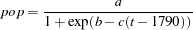 |
where t is time in years. The model is estimated by using decennial census data of the U.S. population in millions. If this simple but highly nonlinear model is estimated by using the default starting values, the estimation fails to converge.
To find reasonable starting values, first consider the meaning of a and c. Taking the limit as time increases, a is the limiting or maximum possible population. So, as a starting value for a, several times the most recent population known can be used—for example, one billion (1000 million).
Dividing the time derivative by the function to find the growth rate and taking the limit as t moves into the past, you can determine that c is the initial growth rate. You can examine the data and compute an estimate of the growth rate for the first few decades, or you can pick a number that sounds like a plausible population growth rate figure, such as 2%.
To find a starting value for b, let t equal the base year used, 1790, which causes c to drop out of the formula for that year, and then solve for the value of b that is consistent with the known population in 1790 and with the starting value of a. This yields  or about 5.5, where a is 1000 and 3.9 is roughly the population for 1790 given in the data. The estimates converge using these starting values.
Convergence Problems
When estimating nonlinear models, you might encounter some of the following convergence problems.
Unable to Improve
The optimization algorithm might be unable to find a step that improves the objective function. If this happens in the Gauss-Newton method, the step size is halved to find a change vector for which the objective improves. In the Marquardt method,  is increased to find a change vector for which the objective improves. If, after MAXSUBITER= step-size halvings or increases in , the change vector still does not produce a better objective value, the iterations are stopped and an error message is printed.
Failure of the algorithm to improve the objective value can be caused by a CONVERGE= value that is too small. Look at the convergence measures reported at the point of failure. If the estimates appear to be approximately converged, you can accept the NOT CONVERGED results reported, or you can try rerunning the FIT task with a larger CONVERGE= value.
If the procedure fails to converge because it is unable to find a change vector that improves the objective value, check your model and data to ensure that all parameters are identified and data values are reasonably scaled. Then, rerun the model with different starting values. Also, consider using the Marquardt method if the Gauss-Newton method fails; the Gauss-Newton method can get into trouble if the Jacobian matrix is nearly singular or ill-conditioned. Keep in mind that a nonlinear model may be well-identified and well-conditioned for parameter values close to the solution values but unidentified or numerically ill-conditioned for other parameter values. The choice of starting values can make a big difference.
Nonconvergence
The estimates might diverge into areas where the program overflows or the estimates might go into areas where function values are illegal or too badly scaled for accurate calculation. The estimation might also take steps that are too small or that make only marginal improvement in the objective function and thus fail to converge within the iteration limit.
When the estimates fail to converge, collinearity diagnostics for the Jacobian crossproducts matrix are printed if there are 20 or fewer parameters estimated. See the section Linear Dependencies for an explanation of these diagnostics.
Inadequate Convergence Criterion
If convergence is obtained, the resulting estimates approximate only a minimum point of the objective function. The statistical validity of the results is based on the exact minimization of the objective function, and for nonlinear models the quality of the results depends on the accuracy of the approximation of the minimum. This is controlled by the convergence criterion used.
There are many nonlinear functions for which the objective function is quite flat in a large region around the minimum point so that many quite different parameter vectors might satisfy a weak convergence criterion. By using different starting values, different convergence criteria, or different minimization methods, you can produce very different estimates for such models.
You can guard against this by running the estimation with different starting values and different convergence criteria and checking that the estimates produced are essentially the same. If they are not, use a smaller CONVERGE= value.
Local Minimum
You might have converged to a local minimum rather than a global one. This problem is difficult to detect because the procedure appears to have succeeded. You can guard against this by running the estimation with different starting values or with a different minimization technique. The START= option can be used to automatically perform a grid search to aid in the search for a global minimum.
Discontinuities
The computational methods assume that the model is a continuous and smooth function of the parameters. If this is not the case, the methods might not work.
If the model equations or their derivatives contain discontinuities, the estimation usually succeeds, provided that the final parameter estimates lie in a continuous interval and that the iterations do not produce parameter values at points of discontinuity or parameter values that try to cross asymptotes.
One common case of discontinuities causing estimation failure is that of an asymptotic discontinuity between the final estimates and the initial values. For example, consider the following model, which is basically linear but is written with one parameter in reciprocal form:
y = a + b * x1 + x2 / c;
By placing the parameter C in the denominator, a singularity is introduced into the parameter space at C=0. This is not necessarily a problem, but if the correct estimate of C is negative while the starting value is positive (or vice versa), the asymptotic discontinuity at 0 will lie between the estimate and the starting value. This means that the iterations have to pass through the singularity to get to the correct estimates. The situation is shown in Figure 18.32.
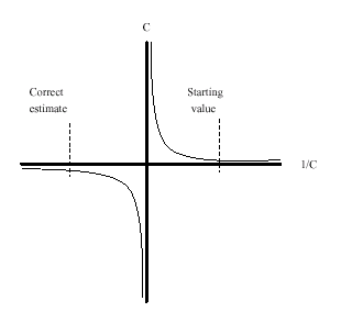
Because of the incorrect sign of the starting value, the C estimate goes off towards positive infinity in a vain effort to get past the asymptote and onto the correct arm of the hyperbola. As the computer is required to work with ever closer approximations to infinity, the numerical calculations break down and an "objective function was not improved" convergence failure message is printed. At this point, the iterations terminate with an extremely large positive value for C. When the sign of the starting value for C is changed, the estimates converge quickly to the correct values.
Linear Dependencies
In some cases, the Jacobian matrix might not be of full rank; parameters might not be fully identified for the current parameter values with the current data. When linear dependencies occur among the derivatives of the model, some parameters appear with a standard error of 0 and with the word BIASED printed in place of the t statistic. When this happens, collinearity diagnostics for the Jacobian crossproducts matrix are printed if the DETAILS option is specified and there are twenty or fewer parameters estimated. Collinearity diagnostics are also printed out automatically when a minimization method fails, or when the COLLIN option is specified.
For each parameter, the proportion of the variance of the estimate accounted for by each principal component is printed. The principal components are constructed from the eigenvalues and eigenvectors of the correlation matrix (scaled covariance matrix). When collinearity exists, a principal component is associated with proportion of the variance of more than one parameter. The numbers reported are proportions so they remain between 0 and 1. If two or more parameters have large proportion values associated with the same principal component, then two problems can occur: the computation of the parameter estimates are slow or nonconvergent; and the parameter estimates have inflated variances (Belsley, Kuh, and Welsch 1980, p. 105–117).
For example, the following cubic model is fit to a quadratic data set:
   proc model data=test3;
      exogenous x1;
      parms b1 a1 c1 ;
      y1 = a1 * x1 + b1 * x1 * x1  + c1 * x1 * x1 *x1;
      fit y1 / collin;
   run;
The collinearity diagnostics are shown in Figure 18.33.
| Collinearity Diagnostics | |||||
|---|---|---|---|---|---|
| Number | Eigenvalue | Condition Number |
Proportion of Variation | ||
| b1 | a1 | c1 | |||
| 1 | 2.942920 | 1.0000 | 0.0001 | 0.0004 | 0.0002 |
| 2 | 0.056638 | 7.2084 | 0.0001 | 0.0357 | 0.0148 |
| 3 | 0.000442 | 81.5801 | 0.9999 | 0.9639 | 0.9850 |
Notice that the proportions associated with the smallest eigenvalue are almost 1. For this model, removing any of the parameters decreases the variances of the remaining parameters.
In many models, the collinearity might not be clear cut. Collinearity is not necessarily something you remove. A model might need to be reformulated to remove the redundant parameterization, or the limitations on the estimability of the model can be accepted. The GINV=G4 option can be helpful to avoid problems with convergence for models containing collinearities.
Collinearity diagnostics are also useful when an estimation does not converge. The diagnostics provide insight into the numerical problems and can suggest which parameters need better starting values. These diagnostics are based on the approach of Belsley, Kuh, and Welsch (1980).
Copyright © 2008 by SAS Institute Inc., Cary, NC, USA. All rights reserved.