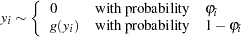
The main motivation for zero-inflated count models is that real-life data frequently display overdispersion and excess zeros. Zero-inflated count models provide a way of modeling the excess zeros as well as allowing for overdispersion. In particular, for each observation, there are two possible data generation processes. The result of a Bernoulli trial is used to determine which of the two processes is used. For observation , Process 1 is chosen with probability and Process 2 with probability . Process 1 generates only zero counts. Process 2 generates counts from either a Poisson or a negative binomial model. In general,

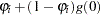
Therefore, the probability of can be described as

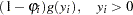where follows either the Poisson or the negative binomial distribution.

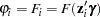
When the probability depends on the characteristics of observation , is written as a function of , where is the vector of zero-inflated covariates and is the vector of zero-inflated coefficients to be estimated. (The zero-inflated intercept is ; the coefficients for the zero-inflated covariates are .) The function relating the product (which is a scalar) to the probability is called the zero-inflated link function,

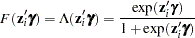
In the COUNTREG procedure, the zero-inflated covariates are indicated in the ZEROMODEL statement. Furthermore, the zero-inflated link function can be specified as either the logistic function,

or the standard normal cumulative distribution function (also called the probit function),

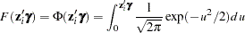The zero-inflated link function is indicated in the ZEROMODEL statement, using the LINK= option. The default ZI link function is the logistic function.