| The AUTOREG Procedure |
| Testing for Heteroscedasticity |
One of the key assumptions of the ordinary regression model is that the errors have the same variance throughout the sample. This is also called the homoscedasticity model. If the error variance is not constant, the data are said to be heteroscedastic.
Since ordinary least squares regression assumes constant error variance, heteroscedasticity causes the OLS estimates to be inefficient. Models that take into account the changing variance can make more efficient use of the data. Also, heteroscedasticity can make the OLS forecast error variance inaccurate since the predicted forecast variance is based on the average variance instead of the variability at the end of the series.
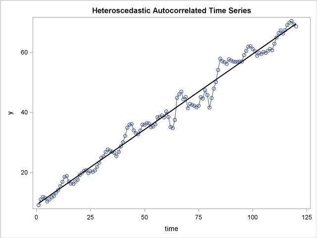
To illustrate heteroscedastic time series, the following statements re-create the simulated series Y. The variable Y has an error variance that changes from 1 to 4 in the middle part of the series. The length of the series is also extended 120 observations.
   data a;
      ul = 0; ull = 0;
      do time = -10 to 120;
         s = 1 + (time >= 60 & time < 90);
         u = + 1.3 * ul - .5 * ull + s*rannor(12346);
         y = 10 + .5 * time + u;
         if time > 0 then output;
         ull = ul; ul = u;
         end;
   run;

   title 'Heteroscedastic Autocorrelated Time Series';
   proc sgplot data=a noautolegend;
      series x=time y=y / markers;
      reg x=time y=y / lineattrs=(color=black);
   run;
The simulated series is plotted in Figure 8.10.
To test for heteroscedasticity with PROC AUTOREG, specify the ARCHTEST option. The following statements regress Y on TIME and use the ARCHTEST option to test for heteroscedastic OLS residuals. The DWPROB option is also used to test for autocorrelation.
   /*-- test for heteroscedastic OLS residuals --*/
   proc autoreg data=a;
      model y = time / nlag=2 archtest dwprob;
      output out=r r=yresid;
   run;
The PROC AUTOREG output is shown in Figure 8.11. The Q statistics test for changes in variance across time by using lag windows ranging from 1 through 12. (See the section Heteroscedasticity and Normality Tests for details.) The p-values for the test statistics are given in parentheses. These tests strongly indicate heteroscedasticity, with p < 0.0001 for all lag windows.
The Lagrange multiplier (LM) tests also indicate heteroscedasticity. These tests can also help determine the order of the ARCH model appropriate for modeling the heteroscedasticity, assuming that the changing variance follows an autoregressive conditional heteroscedasticity model.
| Dependent Variable | y |
|---|
| Heteroscedastic Autocorrelated Time Series |
| Ordinary Least Squares Estimates | |||
|---|---|---|---|
| SSE | 690.266009 | DFE | 118 |
| MSE | 5.84971 | Root MSE | 2.41862 |
| SBC | 560.070468 | AIC | 554.495484 |
| MAE | 3.72760089 | AICC | 554.598048 |
| MAPE | 5.24916664 | Regress R-Square | 0.9814 |
| Durbin-Watson | 0.4060 | Total R-Square | 0.9814 |
| Q and LM Tests for ARCH Disturbances | ||||
|---|---|---|---|---|
| Order | Q | Pr > Q | LM | Pr > LM |
| 1 | 37.5445 | <.0001 | 37.0072 | <.0001 |
| 2 | 40.4245 | <.0001 | 40.9189 | <.0001 |
| 3 | 41.0753 | <.0001 | 42.5032 | <.0001 |
| 4 | 43.6893 | <.0001 | 43.3822 | <.0001 |
| 5 | 55.3846 | <.0001 | 48.2511 | <.0001 |
| 6 | 60.6617 | <.0001 | 49.7799 | <.0001 |
| 7 | 62.9655 | <.0001 | 52.0126 | <.0001 |
| 8 | 63.7202 | <.0001 | 52.7083 | <.0001 |
| 9 | 64.2329 | <.0001 | 53.2393 | <.0001 |
| 10 | 66.2778 | <.0001 | 53.2407 | <.0001 |
| 11 | 68.1923 | <.0001 | 53.5924 | <.0001 |
| 12 | 69.3725 | <.0001 | 53.7559 | <.0001 |
Copyright © 2008 by SAS Institute Inc., Cary, NC, USA. All rights reserved.