The HPSEVERITY Procedure

Example 9.8 Defining a Finite Mixture Model That Has a Scale Parameter

A finite mixture model is a stochastic model that postulates that the probability distribution of the data generation process is a mixture of a finite number of probability distributions. For example, when an insurance company analyzes loss data from multiple policies that are underwritten in different geographic regions, some regions might behave similarly, but the distribution that governs some regions might be different from the distribution that governs other regions. Further, it might not be known which regions behave similarly. Also, the larger amounts of losses might follow a different stochastic process from the stochastic process that governs the smaller amounts of losses. It helps to model all policies together in order to pool the data together and exploit any commonalities among the regions, and the use of a finite mixture model can help capture the differences in distributions across regions and ranges of loss amounts.

Formally, if $f_ i$ and $F_ i$ denote the PDF and CDF, respectively, of component distribution i and $p_ i$ represents the mixing probability that is associated with component i, then the PDF and CDF of the finite mixture of K distribution components are

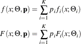
$\begin{align*} f(x; \Theta , \mathbf{p}) & = \sum _{i=1}^{K} p_ i f_ i(x; \Theta _ i) \\ F(x; \Theta , \mathbf{p}) & = \sum _{i=1}^{K} p_ i F_ i(x; \Theta _ i) \end{align*}$

where $\Theta _ i$ denotes the parameters of component distribution i and $\Theta$ denotes the parameters of the mixture distribution, which is a union of all the $\Theta _ i$ parameters. $\mathbf{p}$ denotes the set of mixing probabilities. All mixing probabilities must add up to 1 ( $\sum _{i=1}^{K} p_ i = 1$ ).

You can define the finite mixture of a specific number of components and specific distributions for each of the components by defining the FCMP functions for the PDF and CDF. However, in general, it is not possible to fit a scale regression model by using any finite mixture distribution unless you take special care to ensure that the mixture distribution has a scale parameter. This example provides a formulation of a two-component finite mixture model that has a scale parameter.

To start with, each component distribution must have either a scale parameter or a log-transformed scale parameter. Let $\theta _1$ and $\theta _2$ denote the scale parameters of the first and second components, respectively. Let $p_1 = p$ be the mixing probability, which makes $p_2 = 1-p$ by using the constraint on $\mathbf{p}$ . The PDF of the mixture of these two distributions can be written as

$f(x; \theta _1, \theta _2, \Phi , p) = \frac{p}{\theta _1} f_1(\frac{x}{\theta _1}; \Phi _1) + \frac{1-p}{\theta _2} f_2(\frac{x}{\theta _2}; \Phi _2)$

where $\Phi _1$ and $\Phi _2$ denote the sets of nonscale parameters of the first and second components, respectively, and $\Phi$ denotes a union of $\Phi _1$ and $\Phi _2$ . For the mixture to have the scale parameter $\theta$ , the PDF must be of the form

$f(x; \theta , \Phi ’, p) = \frac{1}{\theta } \left( p f_1(\frac{x}{\theta }; \Phi _1’) + (1-p) f_2(\frac{x}{\theta }; \Phi _2’) \right)$

where $\Phi ’$ , $\Phi _1’$ , and $\Phi _2’$ denote the modified sets of nonscale parameters. One simple way to achieve this is to make $\theta _1 = \theta _2 = \theta$ and $\Phi ’ = \Phi$ ; that is, you simply equate the scale parameters of both components and keep the set of nonscale parameters unchanged. However, forcing the scale parameters to be equal in both components is restrictive, because the mixture cannot model potential differences in the scales of the two components. A better approach is to tie the scale parameters of the two components by a ratio such that $\theta _1 = \theta$ and $\theta _2 = \rho \theta$ . If the ratio parameter $\rho$ is estimated along with the other parameters, then the mixture distribution becomes flexible enough to model the variations across the scale parameters of individual components.

To summarize, the PDF and CDF are of the following form for the two-component mixture that has a scale parameter:

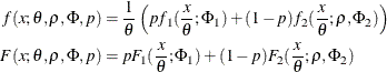
$\begin{align*} f(x; \theta , \rho , \Phi , p) & = \frac{1}{\theta } \left(p f_1(\frac{x}{\theta }; \Phi _1) + (1-p) f_2(\frac{x}{\theta }; \rho , \Phi _2)\right) \\ F(x; \theta , \rho , \Phi , p) & = p F_1(\frac{x}{\theta }; \Phi _1) + (1-p) F_2(\frac{x}{\theta }; \rho , \Phi _2) \end{align*}$

This can be generalized to a mixture of K components by introducing the $K-1$ ratio parameters $\rho _ i$ that relate the scale parameters of each of the K components to the scale parameter $\theta$ of the mixture distribution as follows:

$\begin{align*} \theta _1 & = \theta \\ \theta _ i & = \rho _ i \theta ; \: i \in [2,K] \end{align*}$

In order to illustrate this approach, define a mixture of two lognormal distributions by using the following PDF function:

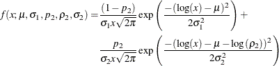
$\begin{align*} f(x;\mu ,\sigma _1,p_2,\rho _2,\sigma _2) = & \frac{(1-p_2)}{\sigma _1 x \sqrt {2\pi }} \exp \left(\frac{-(\log (x) - \mu )^2}{2\sigma _1^2}\right) + \\ & \frac{p_2}{\sigma _2 x \sqrt {2\pi }} \exp \left(\frac{-(\log (x) - \mu - \log (\rho _2))^2}{2\sigma _2^2}\right) \end{align*}$

You can verify that $\mu$ serves as the log of the scale parameter $\theta$ ( $\mu = \log (\theta )$ ).

The following PROC FCMP steps encode this formulation in a distribution named SLOGNMIX2 for use with PROC HPSEVERITY:

/*- Define Mixture of 2 Lognormal Distributions with a Log-Scale Parameter -*/
proc fcmp library=sashelp.svrtdist outlib=work.sevexmpl.models;
   function slognmix2_description() $128;
      return ("Mixture of two lognormals with a log-scale parameter Mu");
   endsub;

   function slognmix2_scaletransform() $8;
      return ("LOG");
   endsub;

   function slognmix2_pdf(x, Mu, Sigma1, p2, Rho2, Sigma2);
      Mu1 = Mu;
      Mu2 = Mu + log(Rho2);
      pdf1 = logn_pdf(x, Mu1, Sigma1);
      pdf2 = logn_pdf(x, Mu2, Sigma2);
      return ((1-p2)*pdf1 + p2*pdf2);
   endsub;

   function slognmix2_cdf(x, Mu, Sigma1, p2, Rho2, Sigma2);
      Mu1 = Mu;
      Mu2 = Mu + log(Rho2);
      cdf1 = logn_cdf(x, Mu1, Sigma1);
      cdf2 = logn_cdf(x, Mu2, Sigma2);
      return ((1-p2)*cdf1 + p2*cdf2);
   endsub;

   subroutine slognmix2_parminit(dim, x[*], nx[*], F[*], Ftype,
                               Mu, Sigma1, p2, Rho2, Sigma2);
      outargs Mu, Sigma1, p2, Rho2, Sigma2;
      array m[1] / nosymbols;
      p2 = 0.5;
      Rho2 = 0.5;
      median = svrtutil_percentile(0.5, dim, x, F, Ftype);
      Mu = log(2*median/1.5);
      call svrtutil_rawmoments(dim, x, nx, 1, m);
      lm1 = log(m[1]);

      /* Search Rho2 that makes log(sample mean) > Mu */
      do while (lm1 <= Mu and Rho2 < 1);
         Rho2 = Rho2 + 0.01;
         Mu = log(2*median/(1+Rho2));
      end;
      if (Rho2 >= 1) then
         /* If Mu cannot be decreased enough to make it less
            than log(sample mean), then revert to Rho2=0.5.
            That will set Sigma1 and possibly Sigma2 to missing.
            PROC HPSEVERITY replaces missing initial values with 0.001. */
         Mu = log(2*median/1.5);

      Sigma1 = sqrt(2.0*(log(m[1])-Mu));
      Sigma2 = sqrt(2.0*(log(m[1])-Mu-log(Rho2)));
   endsub;

   subroutine slognmix2_lowerbounds(Mu, Sigma1, p2, Rho2, Sigma2);
      outargs Mu, Sigma1, p2, Rho2, Sigma2;
      Mu = .; /* Mu has no lower bound */
      Sigma1 = 0; /* Sigma1 > 0 */
      p2 = 0; /* p2 > 0 */
      Rho2 = 0; /* Rho2 > 0 */
      Sigma2 = 0; /* Sigma2 > 0 */
   endsub;

   subroutine slognmix2_upperbounds(Mu, Sigma1, p2, Rho2, Sigma2);
      outargs Mu, Sigma1, p2, Rho2, Sigma2;
      Mu = .; /* Mu has no upper bound */
      Sigma1 = .; /* Sigma1 has no upper bound */
      p2 = 1; /* p2 < 1 */
      Rho2 = 1; /* Rho2 < 1 */
      Sigma2 = .; /* Sigma2 has no upper bound */
   endsub;
quit;

As shown in previous examples, an important aspect of defining a distribution for use with PROC HPSEVERITY is the definition of the PARMINIT subroutine that initializes the parameters. For mixture distributions, in general, the parameter initialization is a nontrivial task. For a two-component mixture, some simplifying assumptions make the problem easier to handle. For the initialization of SLOGNMIX2, the initial values of $p_2$ and $\rho _2$ are fixed at 0.5, and the following two simplifying assumptions are made:

The median of the mixture is the average of the medians of the two components:

$F^{-1}(0.5) = (\exp (\mu _1) + \exp (\mu _2))/2 = \exp (\mu ) (1+\rho _2)/2$

Solution of this equation yields the value of $\mu$ in terms of $\rho _2$ and the sample median.
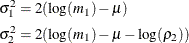
Each component has the same mean, which implies the following:

$\exp (\mu + \sigma _1^2/2) = \exp (\mu + \log (\rho _2) + \sigma _2^2/2)$

If $X_ i$ represents the random variable of component distribution i and X represents the random variable of the mixture distribution, then the following equation holds for the raw moment of any order k:

$E[X^ k] = \sum _{i=1}^{K} p_ i E[X_ i^ k]$

This, in conjunction with the assumption on component means, leads to the equations

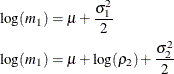
$\begin{align*} \log (m_1) & = \mu + \frac{\sigma _1^2}{2} \\ \log (m_1) & = \mu + \log (\rho _2) + \frac{\sigma _2^2}{2} \end{align*}$

where $m_1$ denotes the first raw moment of the sample. Solving these equations leads to the following values of $\sigma _1$ and $\sigma _2$ :

$\begin{align*} \sigma _1^2 & = 2 (\log (m_1) - \mu ) \\ \sigma _2^2 & = 2 (\log (m_1) - \mu - \log (\rho _2)) \end{align*}$

Note that $\sigma _1$ has a valid value only if $\log (m_1) > \mu$ . Among the many possible methods of ensuring this condition, the SLOGNMIX2_PARMINIT subroutine uses the method of doing a linear search over $\rho _2$ .

Even when the preceding assumptions are not true for a given problem, they produce reasonable initial values to help guide the nonlinear optimizer to an acceptable optimum if the mixture of two lognormal distributions is indeed a good fit for your input data. This is illustrated by the results of the following steps that fit the SLOGNMIX2 distribution to simulated data, which have different means for the two components (12.18 and 22.76, respectively), and the median of the sample (15.94) is not equal to the average of the medians of the two components (7.39 and 20.09, respectively):

/*-------- Simulate a lognormal mixture sample ----------*/
data testlognmix(keep=y);
   call streaminit(12345);
   Mu1 = 2;
   Sigma1 = 1;
   i = 0;
   do j=1 to 2000;
      y = exp(Mu1) * rand('LOGNORMAL')**Sigma1;
      output;
   end;
   Mu2 = 3;
   Sigma2 = 0.5;
   do j=1 to 3000;
      y = exp(Mu2) * rand('LOGNORMAL')**Sigma2;
      output;
   end;
run;

/*-- Fit and compare scale regression models with 2-component  --*/
/*-- lognormal mixture and the standard lognormal distribution --*/
options cmplib=(work.sevexmpl);

proc hpseverity data=testlognmix print=all;
   loss y;
   dist slognmix2 logn;
run;

The comparison of the fit statistics of SLOGNMIX2 and LOGN, as shown in Output 9.8.1, confirms that the two-component mixture is certainly a better fit to these data than the single lognormal distribution.

Output 9.8.1: Comparison of Fitting One versus Two Lognormal Components to Mixture Data

The HPSEVERITY Procedure

All Fit Statistics
Distribution	-2 Log Likelihood		AIC		AICC		BIC		KS		AD		CvM
slognmix2	38343	*	38353	*	38353	*	38386	*	0.52221	*	0.19843	*	0.02728	*
Logn	39073		39077		39077		39090		5.86522		66.93414		11.72703
Note: The asterisk (*) marks the best model according to each column's criterion.

The detailed results for the SLOGNMIX2 distribution are shown in Output 9.8.2. According to the "Initial Parameter Values and Bounds" table, the initial value of $\rho _2$ is not 0.5, indicating that a linear search was conducted to ensure $\log (m_1) > \mu$ .

Output 9.8.2: Detailed Estimation Results for the SLOGNMIX2 Distribution

The HPSEVERITY Procedure

slognmix2 Distribution

Distribution Information
Name	slognmix2
Description	Mixture of two lognormals with a log-scale parameter Mu
Distribution Parameters	5

Initial Parameter Values and Bounds
Parameter	Initial Value	Lower Bound	Upper Bound
Mu	2.92006	-Infty	Infty
Sigma1	0.10455	1.05367E-8	Infty
P2	0.50000	1.05367E-8	1.00000
Rho2	0.72000	1.05367E-8	1.00000
Sigma2	0.81728	1.05367E-8	Infty

Convergence Status
Convergence criterion (GCONV=1E-8) satisfied.

Optimization Summary
Optimization Technique	Trust Region
Iterations	7
Function Calls	18
Log Likelihood	-19171.5

Parameter Estimates
Parameter	Estimate	Standard Error	t Value	Approx Pr > \|t\|
Mu	3.00922	0.01554	193.68	<.0001
Sigma1	0.49516	0.01451	34.13	<.0001
P2	0.40619	0.02600	15.62	<.0001
Rho2	0.37212	0.02038	18.26	<.0001
Sigma2	1.00019	0.02124	47.09	<.0001

By using the relationship that $\mu _2 = \mu + \log (\rho _2)$ , you can see that the final parameter estimates are indeed close to the true parameter values that were used to simulate the input sample.