The HPPANEL Procedure
- Overview
- Getting Started
-
Syntax

-
Details
 Specifying the Input DataSpecifying the Regression ModelSpecifying the Number of Nodes and Number of ThreadsUnbalanced DataOne-Way Fixed-Effects ModelTwo-Way Fixed-Effects ModelBalanced PanelsUnbalanced PanelsOne-Way Random-Effects ModelTwo-Way Random-Effects ModelBetween EstimatorsPooled EstimatorLinear Hypothesis TestingSpecification TestsOUTPUT OUT= Data SetOUTEST= Data SetPrinted OutputODS Table Names
 -
Example

- References
Unbalanced Panels
Let  and
and  be the independent and dependent variables, respectively, that are arranged by time and by cross section within each time
period. (Note that the input data set that the PANEL procedure uses must be sorted by cross section and then by time within
each cross section.) Let
  be the number of cross sections that are observed in year
  , and let
  . Let
. Let  be the
  matrix that is obtained from the
  identity matrix from which rows that correspond to cross sections that are not observed at time
  have been omitted. Consider
![\[ \mb{Z} =(\mb{Z} _{1}, \mb{Z} _{2}) \]](images/etshpug_hppanel0069.png)
where  and
and  . The matrix
  contains the dummy variable structure for the two-way model.
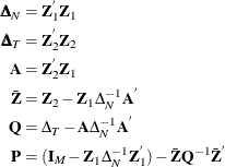
Let

The estimate of the regression slope coefficients is given by
![\[ \tilde{{\beta }}_{s}= ( \mb{X} ^{'}_{{\ast } s}\mb{PX} _{{\ast }s})^{-1} \mb{X} ^{'}_{{\ast } s}\mb{Py} _{{\ast }} \]](images/etshpug_hppanel0074.png)
where  is the
  matrix without the vector of 1s.
The estimator of the error variance is
![\[ \hat{{\sigma }}^{2}_{{\epsilon }}= \tilde{\mb{u} }^{'}\mb{P} \tilde{\mb{u} } / (\mi{M}-\mi{T}-\mi{N} +1-(\mi{K} -1)) \]](images/etshpug_hppanel0077.png)
where the residuals are given by  if there is an intercept in the model and by
  if there is no intercept.
The actual implementation is quite different from the theory. For more information, see the section Two-Way Fixed-Effects Model in SAS/ETS 14.1 User's Guide.