The HPCOUNTREG Procedure

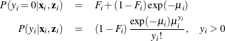
In the zero-inflated Poisson (ZIP) regression model, the data generation process that is referred to earlier as Process 2 is
where ![]() . Thus the ZIP model is defined as
. Thus the ZIP model is defined as
The conditional expectation and conditional variance of ![]() are given by
are given by
Note that the ZIP model (in addition to the ZINB model) exhibits overdispersion because ![]() .
.
In general, the log-likelihood function of the ZIP model is
After a specific link function (either logistic or standard normal) for the probability ![]() is chosen, it is possible to write the exact expressions for the log-likelihood function and the gradient.
is chosen, it is possible to write the exact expressions for the log-likelihood function and the gradient.
First, consider the ZIP model in which the probability ![]() is expressed by a logistic link function, namely
is expressed by a logistic link function, namely
The log-likelihood function is
![\begin{eqnarray*} \mathcal{L} & = & \sum _{\{ i: y_{i}=0\} } \ln \left[\exp (\mathbf{z}_{i}’\bgamma )+\exp (-\exp (\mathbf{x}_{i}’\bbeta )) \right] \\ & & + \sum _{\{ i: y_{i}>0\} }\left[y_{i} \mathbf{x}_{i}’\bbeta -\exp (\mathbf{x}_{i}’\bbeta ) - \sum _{k=2}^{y_{i}}\ln (k) \right] \\ & & - \sum _{i=1}^{N}\ln \left[ 1 + \exp (\mathbf{z}_{i}’\bgamma ) \right] \end{eqnarray*}](images/etshpug_hpcountreg0104.png)
Next, consider the ZIP model in which the probability ![]() is expressed by a standard normal link function:
is expressed by a standard normal link function: ![]() . The log-likelihood function is
. The log-likelihood function is
![\begin{eqnarray*} \mathcal{L} & = & \sum _{\{ i: y_{i}=0\} } \ln \left\{ \Phi (\mathbf{z}_{i}’\bgamma ) + \left[ 1- \Phi (\mathbf{z}_{i}’\bgamma )\right] \exp (-\exp (\mathbf{x}_{i}’\bbeta )) \right\} \\ & + & \sum _{\{ i: y_{i}>0\} } \left\{ \ln \left[ \left( 1-\Phi (\mathbf{z}_{i}’\bgamma )\right) \right] - \exp (\mathbf{x}_{i}’\bbeta ) + y_{i} \mathbf{x}_{i}’\bbeta - \sum _{k=2}^{y_{i}} \ln (k) \right\} \end{eqnarray*}](images/etshpug_hpcountreg0106.png)
For more information about the zero-inflated Poisson regression model, see the section Zero-Inflated Poisson Regression in SAS/ETS 13.2 User's Guide.