Fitting and Comparing Candidate Models
Fitting a Regression Model
On the Model tab,
drag a Regression node to your diagram workspace.
Connect the Interactive Binning node to the Regression
(3) node.
In the Properties Panel,
locate the Model Selection subgroup. These
properties determine whether and which type of model of variable selection
is performed when generating the model. You can choose from the following
variable selection techniques:
-
Backward — Variable selection begins with all candidate effects in the model and systematically removes effects that are not significantly associated with the target. This continues until no other effect in the model meets the Stay Significance Level, or until the Stop Variable Number is met. This method is not recommended for binary or ordinal targets when there are many candidate effects or when there are many levels for some classification input variables.
-
Stepwise — Variable selection begins with no candidate effects in the model and then systematically adds effects that are significantly associated with the target. After an effect is added to the model, it can be removed if it is deemed that the effect is no longer significantly associated with the target.
For this example, set
the value of the Selection Model property
to Forward. Set the value of the Use
Selection Defaults property to No.
After you do this, notice that the Selection Options property
becomes available.
Click  next to the Selection Options property.
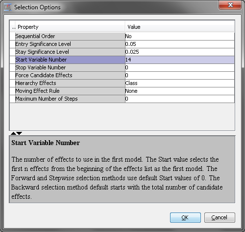
The Selection Options window contains the Entry
Significance Level, Stay Significance Level, Start
Variable Number, and Stop Variable Number properties
that were just mentioned. These properties enable you to control the
significance level required for an effect to remain in or be removed
from a model and the number of effects in a model. For Backward selection,
the Stop Variable Number determines the minimum
number of effects. For Forward selection,
the Stop Variable Number determines the maximum
number of effects.
next to the Selection Options property.
The Selection Options window contains the Entry
Significance Level, Stay Significance Level, Start
Variable Number, and Stop Variable Number properties
that were just mentioned. These properties enable you to control the
significance level required for an effect to remain in or be removed
from a model and the number of effects in a model. For Backward selection,
the Stop Variable Number determines the minimum
number of effects. For Forward selection,
the Stop Variable Number determines the maximum
number of effects.
The Maximum
Number of Steps property enables you to set the maximum
number of steps before the Stepwise method
stops. The default value is twice the number of effects in the model.
The Hierarchy
Effects property determines which variables are subject
to effect hierarchies. Specify Class if you
want to include just the classification variables and All if
you want to use both the classification and interval variables.
Model hierarchy refers
to the requirement that for any effect in the model, all effects that
it contains must also be in the model. For example, in order for the
interaction A*B to be in the model, the main effects A and B must
also be in the model.
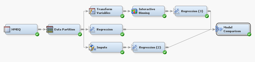
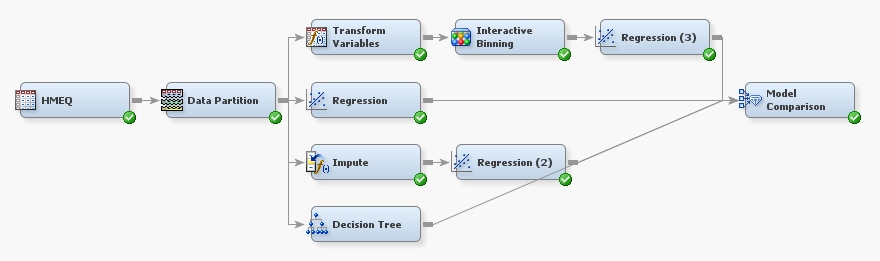
Evaluating the Models
On the Assess tab,
drag a Model Comparison node to your diagram
workspace. Connect the Regression, Regression
(2), and Regression (3) nodes
to the Model Comparison node.
Right-click the Model
Comparison node and click Run.
In the Confirmation window click Yes.
In the Run Status window click Results.
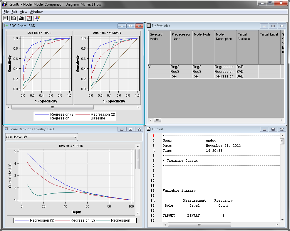
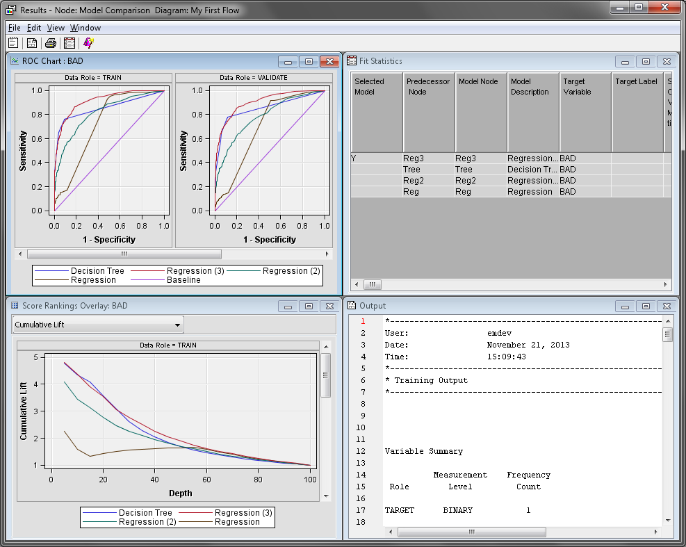
The Model
Comparison node Results window
displays a lift chart that contains all three models. Maximize the Score
Rankings Overlay window. On the drop-down menu, click Cumulative
% Response.
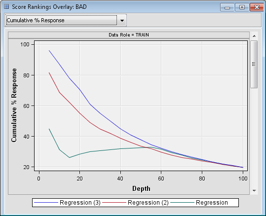
Recall that this chart
groups individuals based on the predicted probability of response,
and then plots the percentage of respondents. Notice that the model
created by the Regression (3) node is better
at almost every depth.
The model created in
the Regression (2) node was created with
no effect selection, because it used the default settings of the Regression
node. Therefore, that model contains every effect.
Maximize the Output window.
Scroll down until you find the Fit Statistics Table.
This table lists all of the calculated assessment statistics for each
model that was compared. Statistics are computed separately for each
partition of the input data. These statistics are also displayed in
the Fit Statistics window.
Fitting a Default Decision Tree
Now that you have modeled
the input data with three different regression models, you want to
fit a tree model to determine whether it will make better predictions.
On the Model tab, drag a Decision
Tree node to your diagram workspace. Connect the Data
Partition node to the Decision Tree node.
Connect the Decision Tree node to the Model
Comparison node.
Tree models handle missing
values differently than regression models, so you can directly connect
the Data Partition node to the Decision
Tree node.
Monotonic transformations
of interval numeric variables are not likely to improve the tree model
because the tree groups numeric variables into bins. In fact, the
tree model might perform worse if you connect it after you group the
input variables. The bins created in the Interactive Binning node
reduce the number of splits that the tree model can consider, unless
you include both the original and binned variables.
Right-click the Model
Comparison node and click Run.
In the Confirmation window, click Yes.
In the Run Status window, click Results.
In the Score
Rankings Overlay window, notice that Cumulative
% Response graphs for the Decision Tree model
and the Regression (3) are fairly similar.
However, the Regression (3) model is better
as the depth increases.
Exploring the Tree Model Results
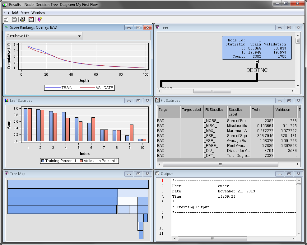
The Tree
Map and Tree windows present
two different views of the decision tree. The Tree window
displays a standard decision tree, where the node splits are provided
on the links between the nodes. Inside the nodes, you can find the
node ID, the training and validation classification rates, and the
number of observations in the node for each partition. The Tree
Map window uses the width of each node to visually display
the percentage of observations in each node on that row. Selecting
a node in one window selects the corresponding node in the other window.
The color of each node
in the decision tree is based on the target variable. The more observations
where BAD=1, the darker the node color is.
The Leaf
Statistics window displays the training and validation
classification rates for each leaf node in the tree model. Leaf nodes
are terminal nodes in the decision tree. Select a bar in the Leaf
Statistics window to select the corresponding leaf node
in the Tree and Tree Map windows.
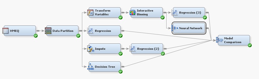
Fitting a Default Neural Network
Next, you want to compare
how well a neural network model compares to the regression and tree
models. On the Model tab, drag a Neural
Network node to your diagram workspace. Connect the Interactive
Binning node to the Neural Network node.
Connect the Neural Network node to the Model
Comparison node.
By default, the Neural
Network node creates a multilayer perceptron (MLP) model
with no direct connections, and the number of hidden layers is data-dependent.
Right-click the Neural
Network node and click Run.
In the Confirmation window, click Yes.
Click Results in the Run Status window.
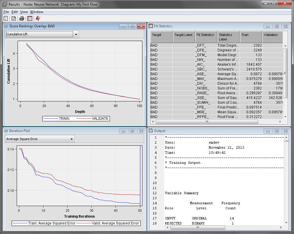
The Fit
Statistics window displays various computed statistics
for the neural network model. The Iteration Plot window
displays various statistics that were computed at each iteration during
the creation of the neural network node.
Explore the rest of
the charts and tables in the Results window.
Close the Results window when you are finished.
In the diagram workspace,
select the Model Comparison node. Right-click
the Model Comparison node and click Run.
In the Confirmation window, click Yes.
In the Run Status window, click Results.
Notice that the predictive
power Neural Network model is very similar
to the Decision Tree and Regression
(3) models. However, both models are considered slightly
better by the Model Comparison node based
on the default assessment criteria. In the Fit Statistics window,
the models are listed in order with best model being at the top of
the table and the worst model at the bottom.
Investigating the Regression and Neural Network Models
The default neural network
model does not perform any better than the regression model. If both
models performed poorly compared to the decision tree model, poor
performance might be due to how missing values are handled. The tree
model directly handles observations with missing values while the
regression and neural network models ignore those observations. This
is why the Regression model is significantly
worse than the Decision Tree model.
In the Neural
Network and Regression (3) model,
you transformed and binned the variables before creating the regression.
When the variables were binned, classification variables were created
and missing values were assigned to a level for each of the new classification
variables.
The Regression
(2) model uses imputation to handle missing values. The
effect of this replacement is that you replace a missing value (perhaps
an unusual value for the variable) with an imputed value (a typical
value for the variable). Imputation can change an observation from
being somewhat unusual with respect to a particular variable to very
typical with respect to that variable.
For example, if someone
applied for a loan and had a missing value for INCOME, the Impute
node would replace that value with the mean value of INCOME by default.
In practice, however, someone who has an average value for INCOME
would often be evaluated differently than someone with a missing value
for INCOME. Any models that follow the Impute node would not be able
to distinguish the difference between these two applicants.
One solution to this
problem is to create missing value indicator variables. These variables
indicate whether an observation originally had a missing value before
imputation is performed. The missing value indicators enable the Regression
and Neural Network nodes to differentiate between observations that
originally had missing values and observations with no missing values.
The addition of missing value indicators can greatly improve a neural
network or regression model.
Recall that you chose
not to use indicator variables earlier. You are going to reverse that
decision now. In your diagram workspace, select the Impute node.
Locate the Type property in the Indicator
Variables subgroup. Set the value of this property to Unique.
Set the value of the Source property to Missing
Values. Set the value of the Role property
to Input.
In the diagram workspace,
select the Model Comparison node. Right-click
the Model Comparison node and click Run.
In the Confirmation window, click Yes.
In the Run Status window, click Results.
Notice that the Regression
(2) model now outperforms the Neural Network model.
In fact, it is the best model in the first decile of the training
data.
In general, it is impossible
to know which model will provide the best results when it is applied
to new data. For this data, or any other, a good analyst considers
many variations of each model and identifies the best model according
to their own criteria. In this case, assume that Regression
(3) is the selected model.
Copyright © SAS Institute Inc. All rights reserved.