Data Preparation and Investigation
Preliminary Investigation
In your process flow
diagram, select the Data Partition node.
You can use the Variables property to access
several summary statistics and statistical graphs for the input data
set. Click the  button next to the Variable property
of the Data Partition node. Select all 13
the variables and click Explore.
button next to the Variable property
of the Data Partition node. Select all 13
the variables and click Explore.
button next to the Variable property
of the Data Partition node. Select all 13
the variables and click Explore.
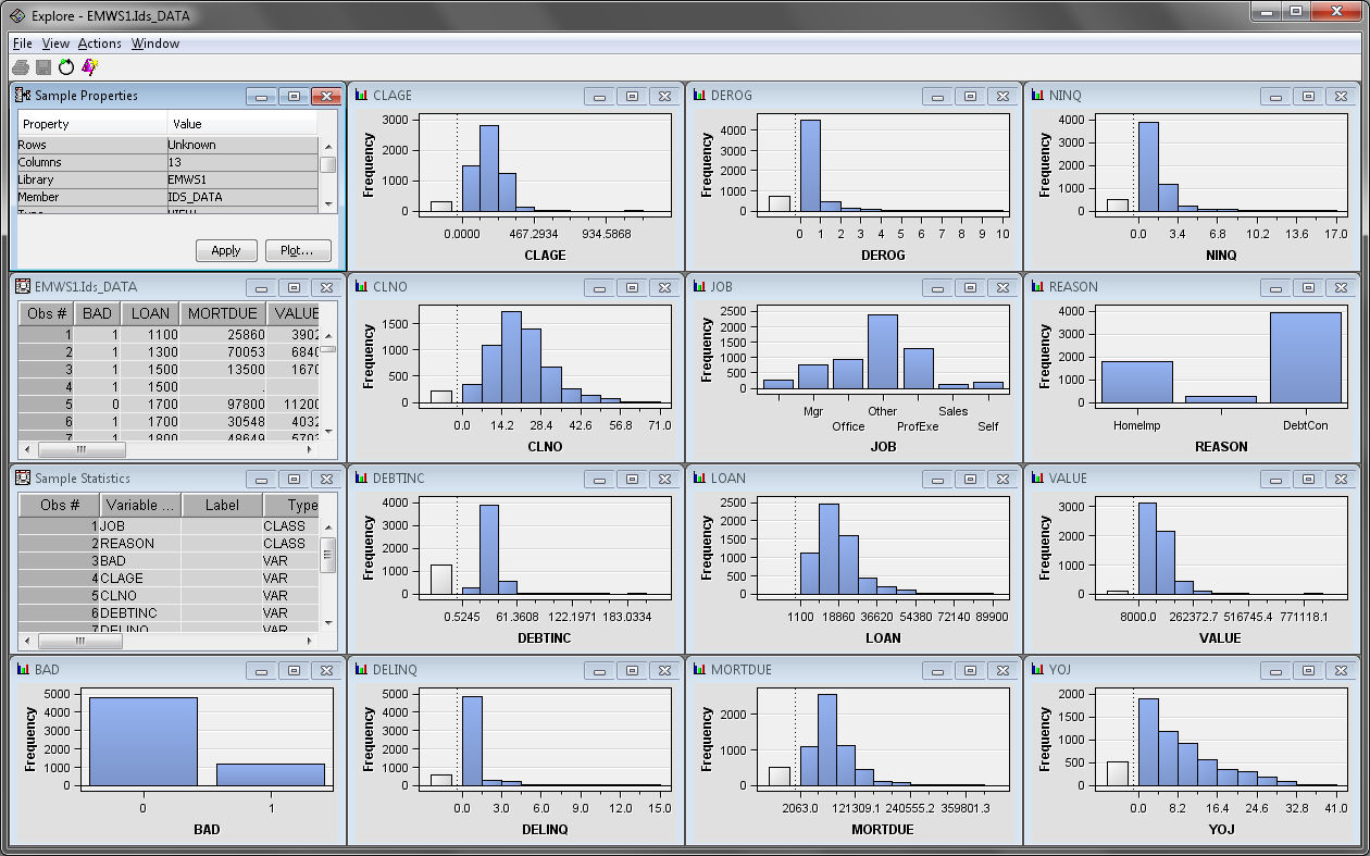
The Explore window
appears. This window contains the sample statistics for every variable,
a histogram for each of the interval variables, and a bar chart for
each class variable. This example highlights only a few of these plots,
but you are encouraged to explore the rest on your own.
Maximize the Sample
Properties window. This window contains information about
the data set sample that was used to create the statistics and graphics
in the Explore window. The Fetched
Rows property indicates the number of observations that
were used in the sample. The SAMPSIO.HMEQ data set is small enough
that the entire data set is used. Close the Sample Properties window.
Maximize the Sample
Statistics window. This window contains the calculated
mean, maximum, and minimum for the interval variables and the number
of class levels, modal value, and percentage of observations in the
modal value for class variables. The percentage of missing values
is calculated for every variable. Close the Sample Statistics window.
Maximize the CLAGE window.
The variable CLAGE indicates the age of the client’s oldest
credit line in months.
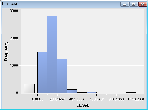
The gray bar on the
left side of the histogram represents the missing values. Notice that
the vast majority of the observations are less than 350. The CLAGE
data set is skewed right. Close the CLAGE window.
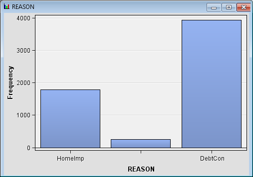
Maximize the REASON window.
This variable represents the stated reason why the client took out
the loan.
Performing Variable Transformation
After you have viewed
the sample statistics and variable distributions, it is obvious that
some variables have highly skewed distributions. In highly skewed
distributions, a small percentage of the data points can have a large
amount of influence on the final model. Sometimes, performing a transformation
on an input variable can yield a better fitting model. The Transform
Variables node enables you to perform variable transformation.
From the Modify tab,
drag a Transform Variables node to your diagram
workspace. Connect the Data Partition node
to the Transform Variables node. Click next to the Variables property
of the Transform Variables node. The Variables window
appears.
next to the Variables property
of the Transform Variables node. The Variables window
appears.
In the Variables window,
select the Statistics option in the upper
right corner of the screen. Scroll the variables list all the way
to the right. You should see the Skewness and Kurtosis statistics.
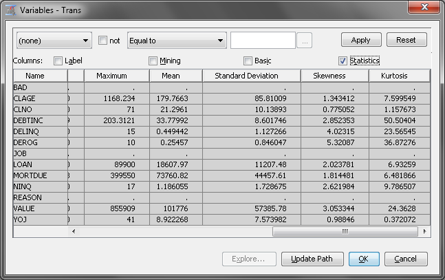
The Skewness statistic
indicates the level of skewness and the direction of skewness for
a distribution. A Skewness value of 0 indicates
that the distribution is perfectly symmetrical. A positive Skewness value
indicates that the distribution is skewed to the right, which describes
all of the variables in this data set. A negative value indicates
that the distribution is skewed to the left.
The Kurtosis statistic
indicates the peakedness of a distribution. However, this example
focuses only on the Skewness statistic.
The Transform
Variables node enables you to rapidly transform interval
variables using standard transformations. You can also create new
variables whose values are calculated from existing variables in the
data set. Note that the most skewed variables are, in order, DEROG,
DELINQ, VALUE, DEBTINC, NINQ, and LOAN. These five variables all have
a Skewness value greater than 2. Close the Variables window.
This example applies
a log transformation to all of the input variables. The log transformation
creates a new variable by taking the natural log of each original
input variable. In your diagram workspace, select the Transform
Variables node. Set the value of the Interval
Inputs property to Log.
Right-click the Transform
Variables property and click Run.
Click Yes in the Confirmation window.
In the Run Status window, click Results.
Maximize the Transformations
Statistics window. This window provides statistics for
the original and transformed variables. The Formula column
indicates the expression used to transform each variable. Notice that
the absolute value of the Skewness statistic
for the transformed values is typically smaller than that of the original
variables. Close the Results window.
The Transform
Variables enables you to perform a different transformation
on each variable. This is useful when your input data contains variables
that are skewed in different ways. In your diagram workspace, select
the Transform Variables node. Click next to the Variables property
of the Transform Variables node. The Variables window
appears. In the Variables window, note the Method column.
Use this column to set the transformation for each variable individually.
next to the Variables property
of the Transform Variables node. The Variables window
appears. In the Variables window, note the Method column.
Use this column to set the transformation for each variable individually.
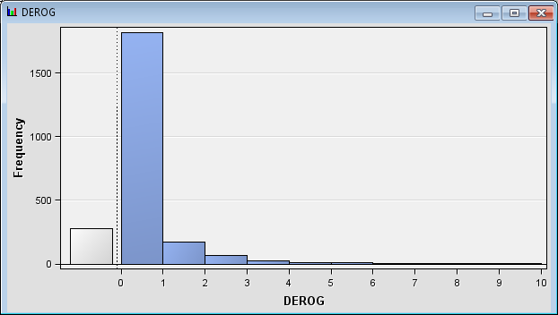
Before doing so, you
want to recall the distribution for each variable. Select the variable DEROG and
click Explore. Note that nearly all of the
observations have a value of 0. Close the Explore window.
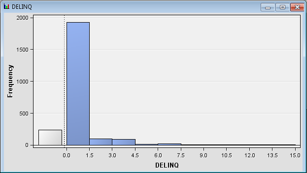
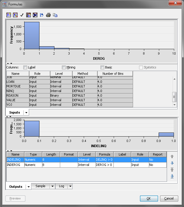
Repeat this process
for the DELINQ variable. Nearly all of the
values for DELINQ are equal to 0. The next largest class is the missing
values.
In situations where
there is a large number of observations at one value and relatively
few observations spread out over the rest of the distribution, it
can be useful to group the levels of an interval variable. Close the Variables window.
Instead of fitting a
slope to the whole range of values for DEROG and DELINQ, you need
to estimate the mean in each group. Because most of the applicants
in the data set had no delinquent credit lines, there is a high concentration
of observations where DELINQ=0.
In your process flow
diagram, select the Transform Variables node.
Click next to the Formulas property.
The Formulas window appears.
next to the Formulas property.
The Formulas window appears.
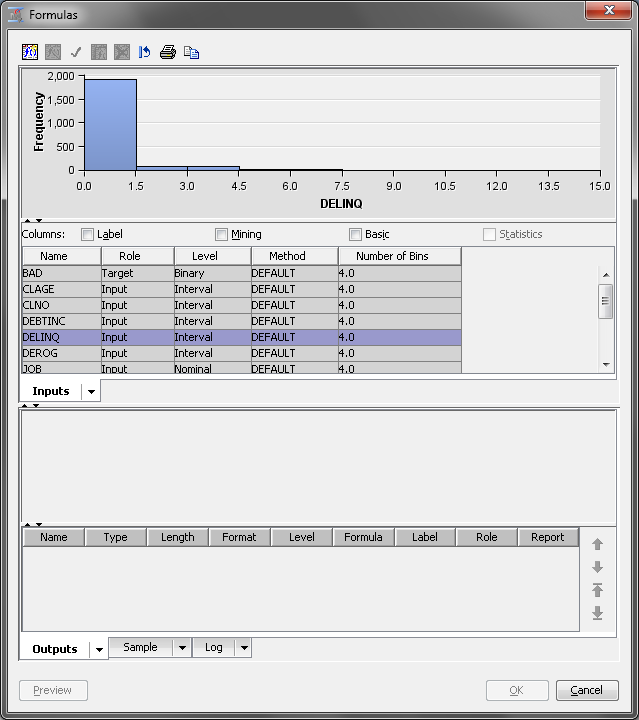
The Formulas window
enables you to create custom variable transformations. Select the DELINQ variable
and click the Create variable in the upper
left corner of the Formulas window. The Add
Transformation window appears.
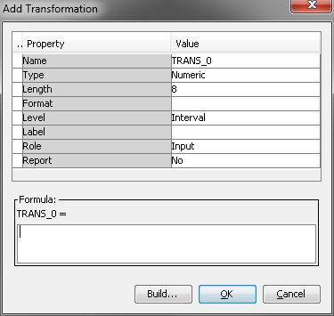
Complete the following
steps to transform the DELINQ variable:
-
This definition is an example of Boolean logic and illustrates one way to dichotomize an interval variable. The statement is either true or false for each observation. When the statement is true, the expression evaluates as 1. Otherwise, the expression evaluates as 0. In other words, when DELINQ>0, INDELINQ=1. Likewise, when DELINQ=0, INDELINQ=0. If the value of DELINQ is missing, the expression evaluates to 0, because missing values are treated as being smaller than any nonmissing values in a numerical comparison. Because a missing value of DELINQ is reasonably imputed as DELINQ=0, this does not pose a problem for this example.
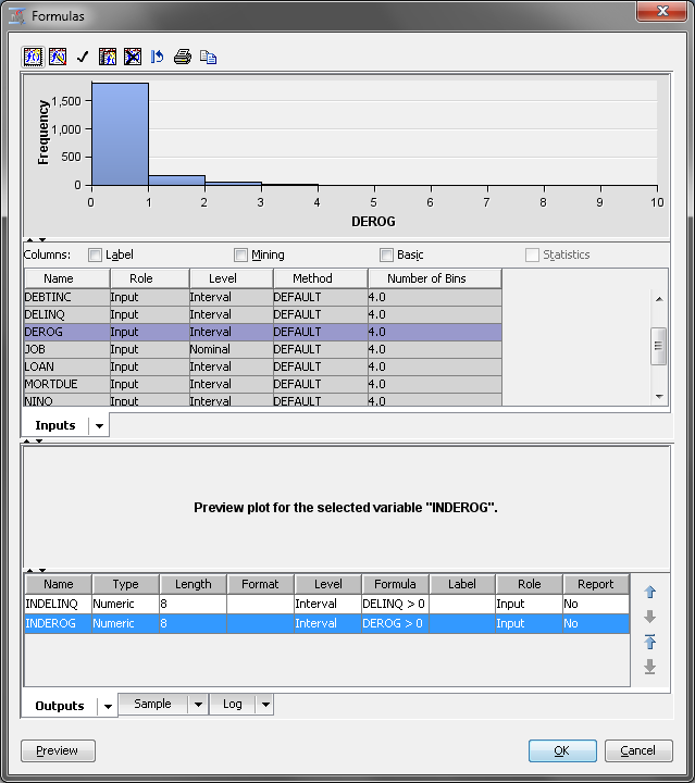
Even though DEROG and
DELINQ were used to construct the new variables, the original variables
are still available for analysis. You can modify this if you want,
but this example keeps the original variables. This is done because
the transformed variables contain only a portion of the information
that is contained in the original variables. Specifically, the new
variables identify whether DEROG or DELINQ is greater than zero.
Understanding Interactive Binning
An additional processing
technique to apply before modeling is binning, also referred to as
grouping. The Interactive Binning node enables you to automatically
group variable values into classes based on the node settings. You
have the option to modify the initially generated classes interactively.
By using the Interactive Grouping node, you can manage the number
of groups of a variable, improve the predictive power of a variable,
select predictive variables, generate the Weight of Evidence (WOE)
for each group of a variable, and make the WOE vary smoothly (or linearly)
across the groups.
The WOE for a group
is defined as the logarithm of the ratio of the proportion of nonevent
observations in the group over the proportion of event observations
in the group. For the binary target variable BAD in this example,
BAD=1 (a client who defaulted) is the event level and BAD=0 (a client
who repaid the loan) is the nonevent level. WOE measures the relative
risk of a group. Therefore, high negative values of WOE correspond
to high risk of loan default. High positive values correspond to low
risk.
After the binning of
variable values has been defined for a variable, you can assess the
predictive power of the variable. The predictive power of a variable
is the ability of the variable to distinguish event and nonevent observations.
In this example, it is the ability to separate bad loan clients from
good loan clients. You can assess the predictive power by using one
of the following criteria:
Performing Interactive Binning
Recall the distribution
of NINQ. NINQ is a counting variable, but the majority of the observations
have the value of either 0, 1, or 2. It might be useful to create
a grouped version of NINQ by pooling all of the values larger than
2 (of which there are very few) into a new level. This would create
a new three-level grouping variable from NINQ. Creating a grouping
variable that has three levels causes loss of information about the
exact number of recent credit inquiries. But it does enable you to
handle nonlinearity in the relationship between NINQ and the response
variable.
In order to bin NINQ,
you need to add an Interactive Binning node
to your process flow diagram. However, because you plan to bin NINQ,
you do not want to transform it with the Transform Variables node.
Right-click the Transform Variables node
and click Variables. Set the value of Method for
the variable NINQ to None. The Transform
Variables node will not transform NINQ.
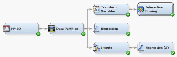
On the Modify tab,
drag an Interactive Binning node to your
process flow diagram. Connect the Transform Variables node
to Interactive Binning node.
Right-click the Interactive
Binning node and click Run. In
the Confirmation window, click Yes.
In the Run Status window, click OK.
In your diagram workspace,
select the Interactive Binning node. Next,
click next to the Interactive Binning property
in the properties panel.
next to the Interactive Binning property
in the properties panel.
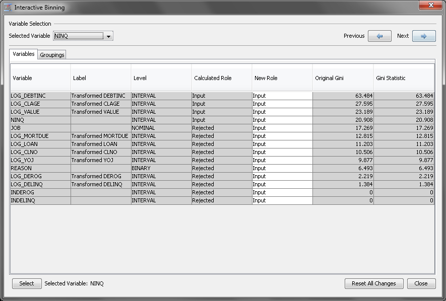
Use the Interactive
Binning window to manually bin the input variables. Before
binning NINQ, first notice that most of the variables have a Calculated
Role of Rejected. Because you
want to use these variables in the data mining process, set their New
Role to Input. To do so, select
all of the variables. Then right-click anywhere in the selection and
click Input. This result is shown in the
image above.
Next, on the Selected
Variable drop-down menu, located in the upper left corner
of the screen, click NINQ. Next, click the Groupings tab
to see details about the variable NINQ.
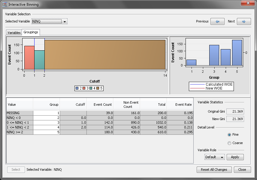
Automatically, the Interactive
Binning node created five groups for NINQ. Notice, however,
that the first two groups contain the missing values and negative
values, respectively. Also notice that the group that contains the
negative values is empty. For this example, you assume that a missing
value indicates that no credit inquiry was made. Therefore, you want
to merge both of these groups into the third group.
First, select the MISSING group
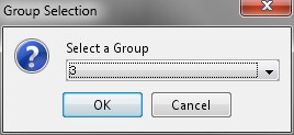
and right-click that row. Click Assign To.
In the Group Selection window, select 3 for
the Select a Group selection.
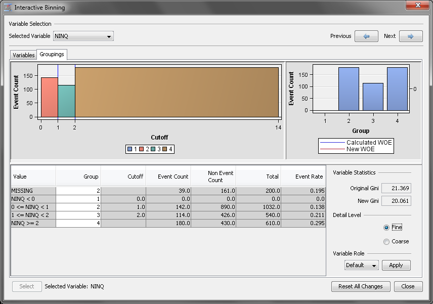
Next, repeat this process
for the empty bin that contains the negative values. Select the group NINQ
< 0 and right-click that row. Click Group
= 2. Once again, this renumbers the groups.
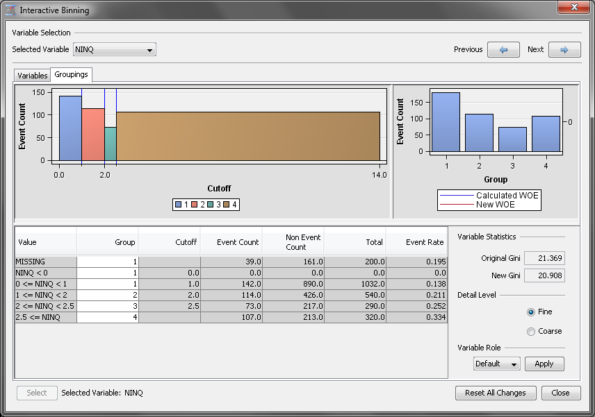
You now have three groups
for the variable NINQ. But you want to add a fourth group that contains
all of the values greater than two and retain a group that contains
just 2. To do so, select the row NINQ >= 2 and
right-click that row. Click Split Bin. Enter
2.5 in
the Enter New Cutoff Value dialog box of Split
Bin window. This creates a separate bin that still belongs
to the same group. To assign this new bin to its own group, right-click
the row 2.5 <= NINQ and click Group
= 4.
Note: Because the values of NINQ
are only whole numbers, you could have selected any value between
2 and 3, exclusive as the new cutoff value.
On the Select
Variable drop-down menu, click INDEROG.
Notice that the Interactive Grouping node decided to split INDEROG
at 0, which means that every observation now belongs to the same bin.
Select the row INDEROG >= 0, right-click
that row and click Split Bin. Enter
0.5 in
the Enter New Cutoff Value dialog box. Click OK.
Now right-click the row 0.5 <= INDEROG and
click GROUP = 4.
You need to repeat this
same process for the variable INDELINQ. On the Select
Variable drop-down menu, click INDELINQ.
Right-click the row INDELINQ >= 0, and
click Split Bin. Enter
0.5 in
the Enter New Cutoff Value dialog box. Click OK.
Now right-click the row 0.5 <= INDELINQ and
click GROUP = 4.
Copyright © SAS Institute Inc. All rights reserved.