Creating a Process Flow Diagram :: Data Mining Using SAS(R) Enterprise Miner(TM): A Case Study Approach, Third Edition

Identifying the Input Data

To begin analyzing HMEQ, you must first add the data source to your project. In the Project Panel, right-click Data Sources and click Create Data Source. This opens the Data Source Wizard. Follow the steps below to complete the Data Source Wizard.

In the Data Source Wizard — Metadata Source window, SAS Table is automatically selected for the Source field. Click Next.
In the Data Source Wizard — Select a SAS Table window, enter SAMPSIO.HMEQ in the Table field. Click Next.
The Data Source Wizard — Table Information window displays some summary information about the HMEQ data set. Click Next.
In the Data Source Wizard — Metadata Advisor Options window, the Basic advisor is automatically selected. Click Next.
In the Data Source Wizard — Column Metadata window, make the following changes to the Role and Level for each variable listed.
- BAD — Set the Role to Target. Set the Level to Binary.
- DELINQ — Set the Level to Ordinal
- REASON — Set the Level to Binary.
Click Next.
In the Data Source Wizard — Decision Configuration window, No is automatically selected. This indicates that SAS Enterprise Miner will not conduct decision processing for this data source. Click Next.
In the Data Source Wizard — Create Sample window, No is automatically selected. This indicates that a sample is not created. Instead, the entire data set is used for analysis. Click Next.
In the Data Source Wizard — Data Source Attributes window, you can rename the data source, change its role, segment the data source, or add notes to the data source. Set the Role of the data source to Train. Click Next.
The Data Source Wizard — Summary window provides a summary of the data source. To create the data source, click Finish.

Adding the Nodes

Begin building the first process flow diagram to analyze this data. Use the SAS Enterprise Miner toolbar to access the nodes that are used in your process flow diagram.

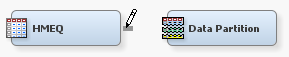
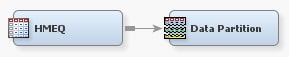
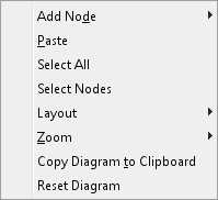
To add the input data, drag the HMEQ data set from the Data Sources section of the Project Panel to the diagram workspace. Because this is a predictive modeling process flow diagram, you will add a Data Partition node. From the Sample tab of the toolbar, drag a Data Partition node to the diagram workspace. You can also add a node by right-clicking in the diagram workspace and selecting Add Node. The nodes in the Add Node menu are grouped in the same categories as the tabs in the toolbar.

Click the Data Partition node to select it. Your process flow diagram should resemble the above image. Note the border around the Data Partition node, which indicates that the node is selected. To deselect every node, click any open space in the project workspace.

Using the Cursor

The cursor shape changes depending on where it is positioned. The behavior of the mouse commands depends on the cursor shape in addition to the selection state of the node over which the cursor is positioned. Right-click in an open area to see the pop-up menu shown below.

When you position the mouse over a node, the cursor becomes a set of intersecting lines. This indicates that you are able to click and drag the node in order to reposition it in the diagram workspace. Note that the node will remain selected after you have placed it in a new location.

The default diagram layout positions the nodes horizontally. This means that the nodes in the process flow diagram run from left to right. You can change the diagram layout to position the nodes vertically by right-clicking the diagram workspace and selecting Layout

Vertically. This selection causes the nodes in the process flow diagram to run from top to bottom.

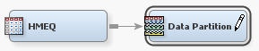
If you position the mouse over the right edge of a node, the cursor will turn into a pencil. This indicates that you can create a connection from this node (the beginning node) to another node (the ending node). To create a connection, position the mouse over the right edge of a beginning node, and then left-click and drag the mouse to the ending node. After the mouse is positioned above the ending node, release the left-click.

Connect your HMEQ node to the Data Partition node.

Understanding the Metadata

All analysis packages must determine how to use variables in the analysis. SAS Enterprise Miner uses metadata in order to make a preliminary assessment of how to use each variable. SAS Enterprise Miner computes simple descriptive statistics that you can access in the Variables window.

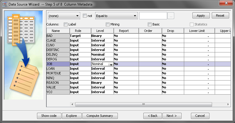
To view the variables and their metadata, right-click the HMEQ node and select Edit Variables. In the Variables window, you can evaluate and update the assignments that were made when the data source was added to your project. The image below shows only the default metadata information. Use the Columns check boxes to view more metadata information for each variable.

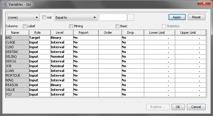
Notice that the column Name has a gray background, which indicates that you cannot edit the values in this column. Variable names must conform to the same naming standards that were described earlier for libraries.

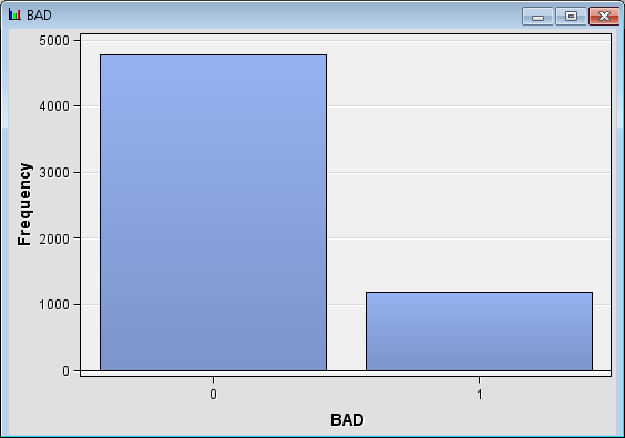
The first variable listed is BAD. Although BAD is a numeric variable, it is assigned the Level of Binary because it has only two distinct nonmissing values.

The variables LOAN, MORTDUE, and VALUE are assigned the Level of Interval because they are numeric variables with more than 10 distinct values.

The variables REASON and JOB are both character variables. However, you set their Level to different values. Because REASON has only two distinct, nonmissing values, it is best modeled as a Binary variable. JOB is best modeled as a Nominal variable because it is a character variable with more than two distinct, non-missing values.

Two other values for Level are available, Unary and Ordinal. A unary variable is a variable that has only one value. An ordinal variable is a numeric variable where the relative order of each value is important. SAS Enterprise Miner automatically assigns numeric variables with more than 2 and fewer than 10 unique values a Level of Ordinal. Ordinal variables often contain counts, such as the number of children.

Inspecting Distribution

You can inspect the distribution of values in the input data set for each variable. To view the distribution for the variable BAD, complete the following steps:

In the Variables window, select the variable BAD.
Click the Explore icon on the bottom right corner of the screen.
The Explore window appears. The BAD window displays the distribution of the variable BAD.

On the bar chart, you can see that approximately 80% of the observations in BAD have a value of 0 and 20% have a value of 1. This means that approximately 20% of the customers in this sample data set defaulted on their loans.
Close the Explore window and the Variables window.

Investigating Descriptive Statistics

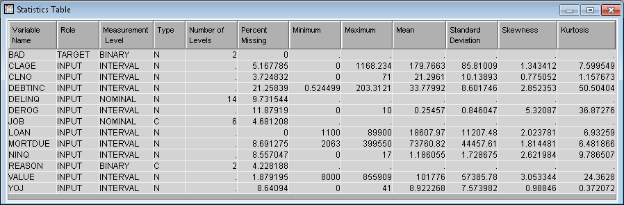
Use the HMEQ data source to calculate and explore descriptive statistics for the input data. To do so, complete the following steps:

In your project workspace, select the HMEQ data source.
Set the value of the Summarize property to Yes.
Right-click the HMEQ data source and click Run. In the Confirmation window, click Yes. After the node has successfully run, click Results in the Run Status window.
The Results window appears. The Statistics Table table window contains the descriptive statistics.

Investigate the minimum value, maximum value, mean, standard deviation, percentage of missing values, number of levels, skewness, and kurtosis of the variables in the input data. In this example, there does not appear to be any unusual minimum or maximum values. Notice that, at approximately 22%, DEBTINC has a high percentage of missing values.
Close the Results window.

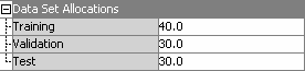
Inspecting the Default Settings of the Data Partition Node

In your diagram workspace, select the Data Partition node. The default Partitioning Method for the Data Partition node is stratified because BAD is a class variable. The available methods for partitioning are as follows:

Simple Random — Every observation in the data set has the sample probability to be selected for a specific partition.
Stratified — When you use stratified partitioning, specific variables form strata (or subgroups) of the total population. Within each stratum, all observations have an equal probability of being assigned to one of the partitioned data sets.
Cluster — When you use cluster partitioning, distinct values of the cluster variable are assigned to the various partitions using simple random partitioning. Note that with this method, the partition percentages apply to the values of the cluster variable, and not to the number of observations that are in the partition data sets

Use the Random Seed property to specify the seed value for random numbers that generated to create the partitions. If you use the same data set and the same Random Seed, excluding the seed value 0, in different process flow diagrams, your partitioning results will be identical. Note that re-sorting the data results in a different ordering of the data, and there a different partitioning of the data. This can lead to slightly different modeling results.

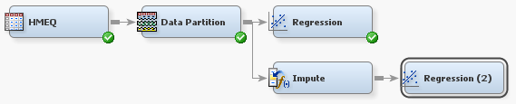
The Data Set Allocations property subgroup enables you to specify what percentage of the input data set is included in each partition. These values must sum to 100.

For this example, use the default settings.

Fitting and Evaluating a Regression Model with Data Replacement

Now that you have decided how the input data is partitioned, you are ready to add a modeling node to the process flow diagram. On the Model tab, drag a Regression node to the diagram workspace. Connect the Data Partition node to the Regression node.

Modeling nodes, such as the Regression node, require a target variable. The Regression node fits models for interval, ordinal, nominal, and binary target variables. Because the target variable BAD is a binary variable, the default model is a binary logistic regression model with main effects for each input variable. By default, the node codes your grouping variables with deviation coding. You can specify GLM coding if desired.

In your process flow diagram, right-click the Regression node and click Run. In the Confirmation window, click Yes. After the node has successfully run, click Results in the Run Status window.

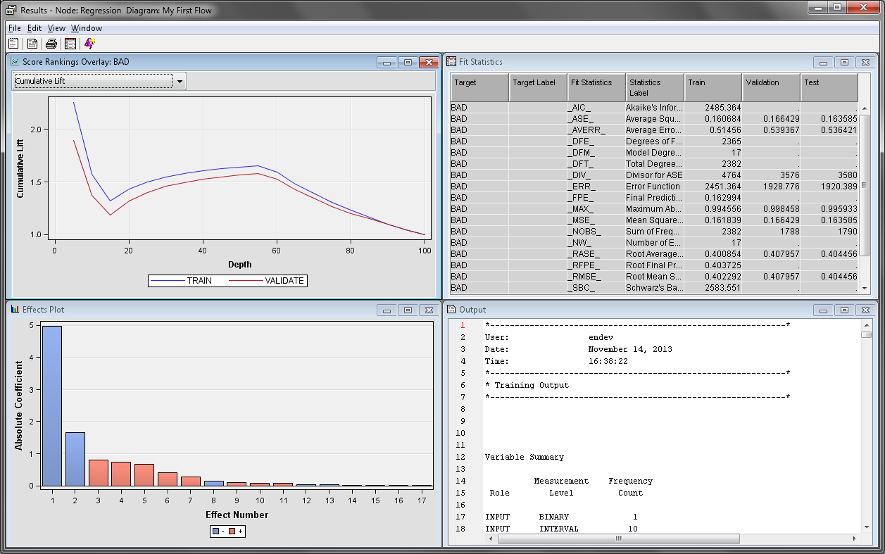
The Effects Plot window contains a bar chart of the absolute value of the model effects. The greater the absolute value, the more important that variable is to the regression model. In this example, the most important variables, and thus best predictor variables, are DELINQ, JOB, NINQ, and DEROG.

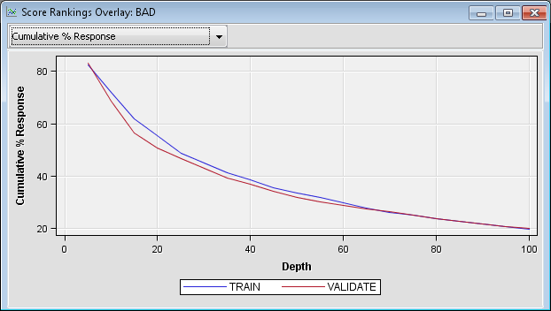
The Score Rankings Overlay window enables you to view assessment charts. The default chart is the Cumulative Lift chart. Open the drop-down menu in the upper left corner of the Score Rankings Overlay window and click Cumulative % Response. This chart arranges the observations into deciles based on their predicted probability of response. It then plots the actual percentage of respondents.

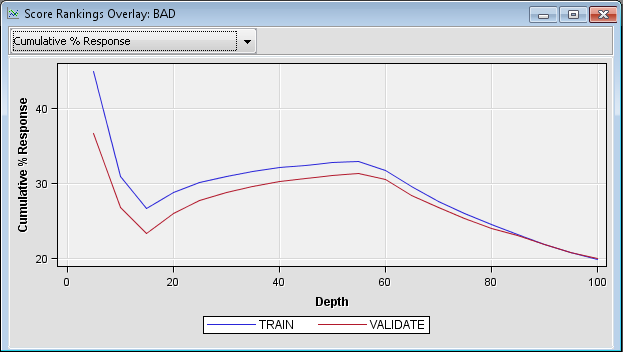
In this example, the individuals are sorted in descending order of their predicted probability of defaulting on a loan. The plotted values are the cumulative actual probabilities of loan defaults. The Score Rankings Overlay window displays information for both the training and the validation data sets. If the model is useful, the proportion of individuals that defaulted on a load is relatively high in the top deciles and the plotted curve is decreasing. Because this curve steadily increases throughout the middle deciles, the default regression model is not useful.

Recall that the variable DEBTINC has a high percentage of missing values. Because of this, it is not appropriate to apply a default regression model directly to the training data. Regression models ignore observations that have a missing value for at least one input variable. Therefore, you should consider variable imputation before fitting a regression model. Use the Impute node to impute missing values in the input data set.

Understanding Data Imputation

The Impute node enables you to impute missing values in the input data set. Imputation is necessary to ensure that every observation in the training data is used when you build a regression or neural network model. Tree models are able to handle missing values directly. But regression and neural network models ignore incomplete observations. It is more appropriate to compare models that are built on the same set of observations. You should perform variable replacement or imputation before fitting any regression or neural network model that you want to compare to a tree model.

The Impute node enables you to specify an imputation method that replaces every missing value with some statistic. By default, interval input variables are replaced by the mean of that variable. Class input variables are replaced by the most frequent value for that variable. This example will use those default values.

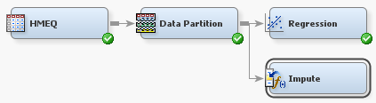
On the Modify tab, drag an Impute node to your diagram workspace. Connect the Data Partition node to the Impute node as shown in the diagram below.

The default imputation method for class variables is Count. This means that missing values are assigned the modal value for each variable. If the modal value is missing, then SAS Enterprise Miner uses the second most frequently occurring level.

The complete set of imputation methods for class variables is as follows:

Count — Use the Count setting to replace missing class variable values with the most frequently occurring class variable value.
Default Constant Value — Use the Default Constant setting to replace missing class variable values with the value that you enter in the Default Character Value property.
Distribution — Use the Distribution setting to replace missing class variable values with replacement values that are calculated based on the random percentiles of the variable's distribution. In this case, the assignment of values is based on the probability distribution of the nonmissing observations. The distribution imputation method typically does not change the distribution of the data very much.
Tree — Use the Tree setting to replace missing class variable values with replacement values that are estimated by analyzing each input as a target. The remaining input and rejected variables are used as predictors. Use the Variables window to edit the status of the input variables. Variables that have a model role of target cannot be used to impute the data. Because the imputed value for each input variable is based on the other input variables, this imputation technique might be more accurate than simply using the variable mean or median to replace the missing tree values.
Tree Surrogate — Use the Tree Surrogate setting to replace missing class variable values by using the same algorithm as Tree Imputation, except with the addition of surrogate splitting rules. A surrogate rule is a backup to the main splitting rule. When the main splitting rule relies on an input whose value is missing, the next surrogate is invoked. If missing values prevent the main rule and all the surrogates from applying to an observation, the main rule assigns the observation to the branch that is assigned to receive missing values.
None — Missing class variable values are not imputed under the None setting.

The following imputation methods are available for interval target variables:

Mean — Use the Mean setting to replace missing interval variable values with the arithmetic average, calculated as the sum of all values divided by the number of observations. The mean is the most common measure of a variable's central tendency. It is an unbiased estimate of the population mean. The mean is the preferred statistic to use to replace missing values if the variable values are at least approximately symmetric (for example, a bell-shaped normal distribution). Mean is the default setting for the Default Input Method for interval variables.
Median — Use the Mean setting to replace missing interval variable values with the 50th percentile, which is either the middle value or the arithmetic mean of the two middle values for a set of numbers arranged in ascending order. The mean and median are equal for a symmetric distribution. The median is less sensitive to extreme values than the mean or midrange. Therefore, the median is preferable when you want to impute missing values for variables that have skewed distributions. The median is also useful for ordinal data.
Midrange — Use the Midrange setting to replace missing interval variable values with the maximum value for the variable plus the minimum value for the variable divided by two. The midrange is a rough measure of central tendency that is easy to calculate.
Distribution — Use the Distribution setting to replace missing interval variable values with replacement values that are calculated based on the random percentiles of the variable's distribution. The assignment of values is based on the probability distribution of the nonmissing observations. This imputation method typically does not change the distribution of the data very much.
Tree — Use the Tree setting to replace missing interval variable values with replacement values that are estimated by analyzing each input as a target. The remaining input and rejected variables are used as predictors. Use the Variables window to edit the status of the input variables. Variables that have a model role of target cannot be used to impute the data. Because the imputed value for each input variable is based on the other input variables, this imputation technique might be more accurate than simply using the variable mean or median to replace the missing tree values.
Tree Surrogate — Use the Tree Surrogate setting to replace missing interval variable values by using the same algorithm as Tree Imputation, except with the addition of surrogate splitting rules. A surrogate rule is a backup to the main splitting rule. When the main splitting rule relies on an input whose value is missing, the next surrogate is invoked. If missing values prevent the main rule and all the surrogates from applying to an observation, the main rule assigns the observation to the branch that is assigned to receive missing values.
Mid-Minimum Spacing — Use the Mid-Minimum setting to replace missing interval variable values with mid-minimum spacing. The mid-minimum spacing method uses a numeric constant to specify the proportion of the data to be contained in the spacing.
Tukey's Biweight — Use the Tukey's Biweight setting to replace missing interval variable values with the Tukey's Biweight robust M-estimator value.
Huber — Use the Huber setting to replace missing interval variable values with the Huber's robust M-estimator value.
Andrew's Wave — Use the Andrew's Wave setting to replace missing interval variable values with the Andrew's Wave robust M-estimator value.
Default Constant — Use the Default Constant Value setting to replace missing interval variable values with the value that you enter in the Default Character Value property.
None — Specify the None setting if you do not want to replace missing interval variable values.

Select the Impute node and find the Indicator Variables property subgroup in the properties panel. Set the value of Type to Single to create a single indicator variable that indicates whether any variable was imputed for each observation. Set the value of Type to Unique to create an indicator variable for each original variable that identifies if that specific variable was imputed.

For this example, set the value of Type to None.

An indicator variable is a special variable that is created automatically by SAS Enterprise Miner. The value of this variable is 1 when an observation contained a missing value and 0 otherwise. The Regression and Neural Network nodes can use the indicator variables to identify observations that had missing values before the imputation.

Fitting and Evaluating a Regression Model with Data Imputation

Next, you will build a new regression model based on the imputed data set. From the Model tab, drag a Regression node to your diagram workspace. Connect the Impute node to the new Regression node.

Right-click the Regression (2) node and click Run. In the Confirmation window, click Yes. After the node has successfully run, click Results in the Run Status window.

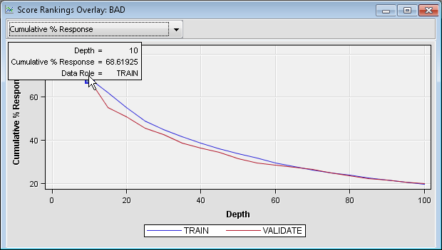
In the Score Rankings Overlay window, click Cumulative % Response on the drop-down menu in the upper left corner. Notice that this model shows a smooth decrease in the cumulative percent response, which contrasts with the previous model. This indicates that the new model is much better than the first model at predicting who will default on a loan.

The discussion of the remaining charts refers to those who defaulted on a loan as defaults or respondents. This is because the target level of interest is BAD=1.

Position the mouse over a point on the Cumulative % Response plot to see the cumulative percent response for that point on the curve. Notice that at the first decile (the top 10% of the data), approximately 69% of the loan recipients default on their loan.

On the drop-down menu in the upper left corner of the Score Rankings Overlay window, click % Response. This chart shows the non-cumulative percentage of loan recipients that defaulted at each level of the input data.

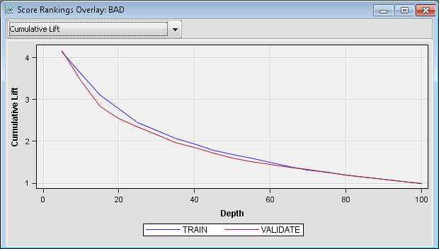
On the drop-down menu, click Cumulative Lift.

Lift charts plot the same information about a different scale. As discussed earlier, the overall response rate is approximately 20%. You calculate lift by dividing the response rate in a given group by the overall response rate. The percentage of respondents in the first decile was approximately 69%, so the lift for that decile is approximately 69/20 = 3.45. Position the cursor over the cumulative lift chart at the first decile to see that the calculated lift for that point is 3.4. This indicates that the response rate in the first decile is more than three times greater than the response rate in the population.

Instead of asking the question, “What percentage of those in a bin were defaulters?”, you could ask the question, “What percentage of the total number of defaulters are in a bin?” The latter question can be evaluated by using the Cumulative % Captured Response curve. Click Cumulative % Captured Response on the drop-down menu.

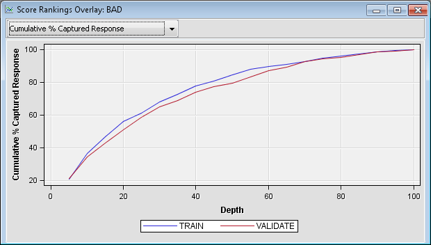
You can calculate lift from this chart as well. If you were to take a random sample of 10% of the observations, you would expect to capture 10% of the defaulters. Likewise, if you take a random sample of 20% of the data, you would expect to capture 20% of the defaulters. To calculate lift, divide the proportion of the defaulters that were captured by the percentage of those whom you have chosen for action (rejection of the loan application).

Note that at the 20th percentile, approximately 55% of those who defaulted are identified. At the 30th percentile, approximately 68% of those who defaulted are identified. The corresponding lift values for those two percentiles are approximately 2.75 and 2.27, respectively. Observe that lift depends on the proportion of those who have been chosen for action. Lift generally decreases as you choose larger proportions of the data for action. When you compare two models on the same proportion of the data, the model that has the higher lift is often preferred, excluding issues that involve model complexity and interpretability.

Note: A model that performs best in one decile might perform poorly in other deciles. Therefore, when you compare competing models, your choice of the final model might depend on the proportion of individuals that you have chosen for action.

As with the initial Regression node results, you can view the Effects Plot for this model. Note that in this model, the most important variables are DELINQ, JOB, DEROG, NINQ, and REASON.