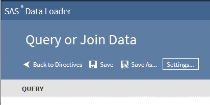
Query or Join Data
Introduction
Use
queries to group rows based on the values in one or more columns and
then summarize selected numeric columns. The summary data appears
in new columns in the target table. You can also filter rows, sort
columns, select and revise columns, and use expressions to modify
data or add new columns.
Use joins to combine
source tables. The join is based on a comparison of values in “join-on”
columns that are selected for each of the source tables. The result
of the join depends on matching values in the join-on columns, and
on the selected type of the join. Four types of joins are available:
inner, left, right, and full.
The Query or Join Data
directive enables you to create jobs that execute a single query or
join, or combine multiple joins. In the resulting table, you can remove
unwanted rows and columns, remove duplicate rows, and rearrange columns.
Before you execute the job, you can edit the generated SQL code and
paste-in additional SQL code. The process of the directive is defined
as follows:
-
Select a source table.
-
Join tables to the initial table as needed.
-
Define summarizations that group columns and aggregate numeric values, again as needed.
-
Use rules or expressions to filter unwanted rows from the target.
-
Select, rename, rearrange, and change type and length of target columns.
-
Apply SQL expressions to modify existing columns or add data to new columns.
-
Sort target rows based on specified target columns.
Enable the Cloudera Impala SQL Environment
Support for the Cloudera
Impala SQL environment is enabled in the Hadoop Configuration panel
of the Configuration window. When Impala
is enabled, new instances of the following directives use the Cloudera
Impala SQL environment by default:
The default SQL environment can be overridden using
the Settings menu. To learn more about SQL
environments, see Enable Support for Impala and Spark.
-
Query or Join
-
Sort and De-Duplicate
-
Run a Hadoop SQL Program
Note: Changing the default SQL
environment does not change the SQL environment for saved directives.
Saved directives continue to run with their existing SQL environment
unless they are opened, reconfigured, and saved.
Example
Follow these steps to
use the Query or Join Data directive.
-
On the SAS Data Loader directives page, click Query or Join Data.
-
In the Query task, click the browse icon
 .
.
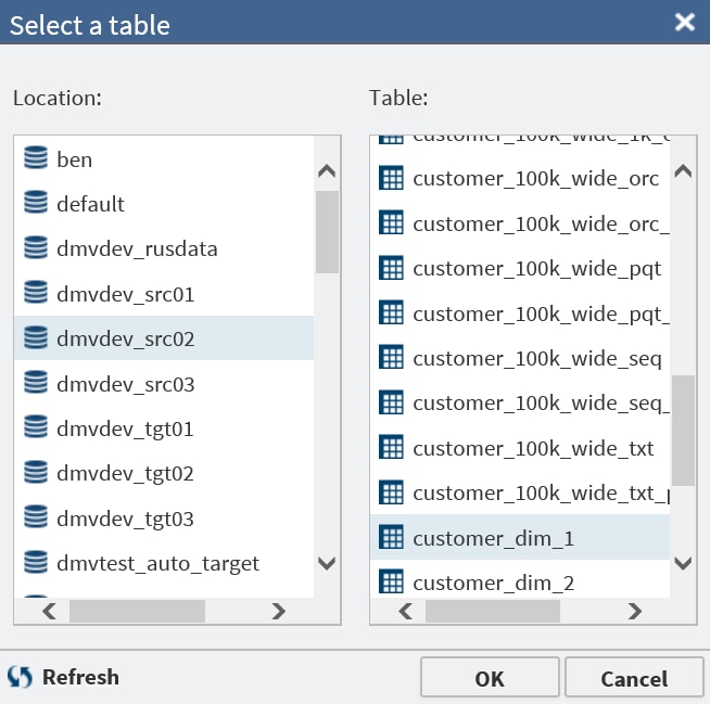
-
In the Select a Table window, scroll through the Location list and click a schema. Then click a source table in the Table list, and then click OK.
-
If your job includes no joins, click Next to open the Summarize Rows task.
-
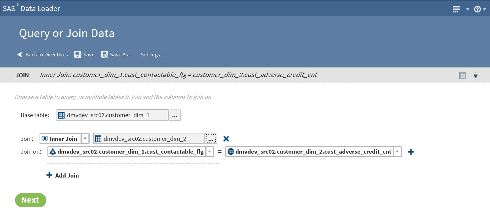
To join your source table with other tables, click Add Join, and then click Next.
-
In the Join row, click the browse icon and select the table for the join.
-
As needed, click the Join field and select a join type other than the default join type Inner.InnerThe inner join finds matching values in the join-on columns and writes one row to the target. The target row contains all columns from both source tables. A row from either source table is not written to the target if it contains a null value in the join-on column. A row is also not written to the target if the value in the join-on column does not match a value in the join-on column in the other source table.LeftThe left or left-full join writes to the target all rows from the left table of the join statement. If a match does not exist between the join-on columns, null values are written to the target for the columns of the right table in the join.RightThe right or right-full join reverses the definition of the left join. All rows from the right table appear in the target. If no values match between the join-on columns, then null values are written to the target for the columns of the table on the left side of the join statement.FullThe full join combines the left and right joins. If a match exists between the join-on columns, then a single row is written to the target to represent those two source rows. If the left or right table has a value in the join-on column that does not match, then the data for that row is written to the target. Null values are written into the columns from the other source table.
-
In the Join-on row, click the left join-on column and select a replacement for the default column, as needed.
 Note: The left and right designations in the join-on statement define the output that is generated by the available left join and right join.
 -
Click the right join-on column to select a replacement for the column, as needed.
-
To add more join columns, click the Add icon
 at the end of the Join-on row.
A match between the source tables consists of a match in the first
pair of join-on values and a match between
the second pair of join-on values.
at the end of the Join-on row.
A match between the source tables consists of a match in the first
pair of join-on values and a match between
the second pair of join-on values.
-
To join a third table to the joined table that unites the two source tables, click Add join.
-
Click Next and wait a moment while the application assembles in memory the names of the joined columns.
-
In the Summarize Rows task, if you do not need to summarize, click Next.Note: If your source data is in Hive 13 (0.13.0 or lower,) the Summarize Rows task will not handle special characters in column names. To resolve the issue, either rename the columns or ask your Hadoop administrator to upgrade to Hive 14 (0.14.0 or higher.)
-
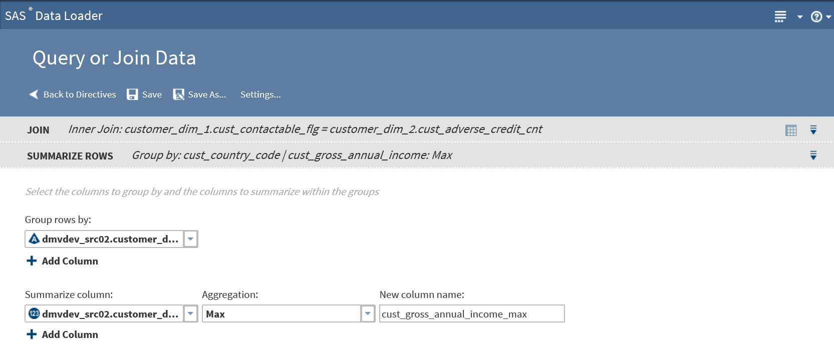
To add summarizations, click the Group rows by field, and then click the column that you want to use as the primary grouping in your target table. For example, if you are querying a table of product sales data, then you could group rows by the product type column.Note:
-
If your job includes joins, note that the Group rows by list includes all columns from your source tables.
-
If you intend to paste an SQL query (HiveQL or Cloudera Impala SQL) into this directive, then you can click Next two times to display the Code task.
-
-
To subset the first group with a second group, and to generate a second set of aggregations, click Add column.
-
To generate multiple aggregations, you can add additional groups. The additional groups will appear in the target table as nested subgroups. Each group that you define will receive its own aggregations.To add a group, click Add Column, and then repeat the previous step to select a different column than the first group. In a table of product sales data, you could choose a second group by selecting the column product_code.
-
In Summarize columns, select the first numeric column that you want to aggregate.
-
In Aggregation, select one of the following:Countspecifies the number of rows that contain values in each group.Count Distinctspecifies the number of rows that contain distinct (or unique) values in each group.Maxspecifies the largest value in each group.Minspecifies the smallest value in each group.Sumspecifies the total of the values in each group.
-
In New column name, either accept the default name of the aggregation column, or click to specify a new name.
-
To add an aggregation, click Add Column.
-
When the aggregations are complete, click Next.
-
In the Filter Data task, all source rows are included in the target by default. To accept this default, click Next.
-
If your job includes no summarizations, then you can select No duplicate rows to remove duplicate rows from the target.Note: If Hive is enabled for this directive, note that older versions of Hive do not support the selection of both No duplicate rows and All Rows.
-
To filter rows from the target, choose one of the following:
-
To filter rows using one or more rules, click Specify rules and proceed to the next step. You can specify multiple rules and apply them using logical AND and OR operators.
-
To filter rows using an expression, click Specify expression and go to Step 26.
-
-
To filter rows by specifying one or more rules, follow these steps:
-
Click Select a column and choose the source column that forms the basis of your rule.
-
Click and select a logical Operator. The operators that are available depend on the type of the data in the source column.
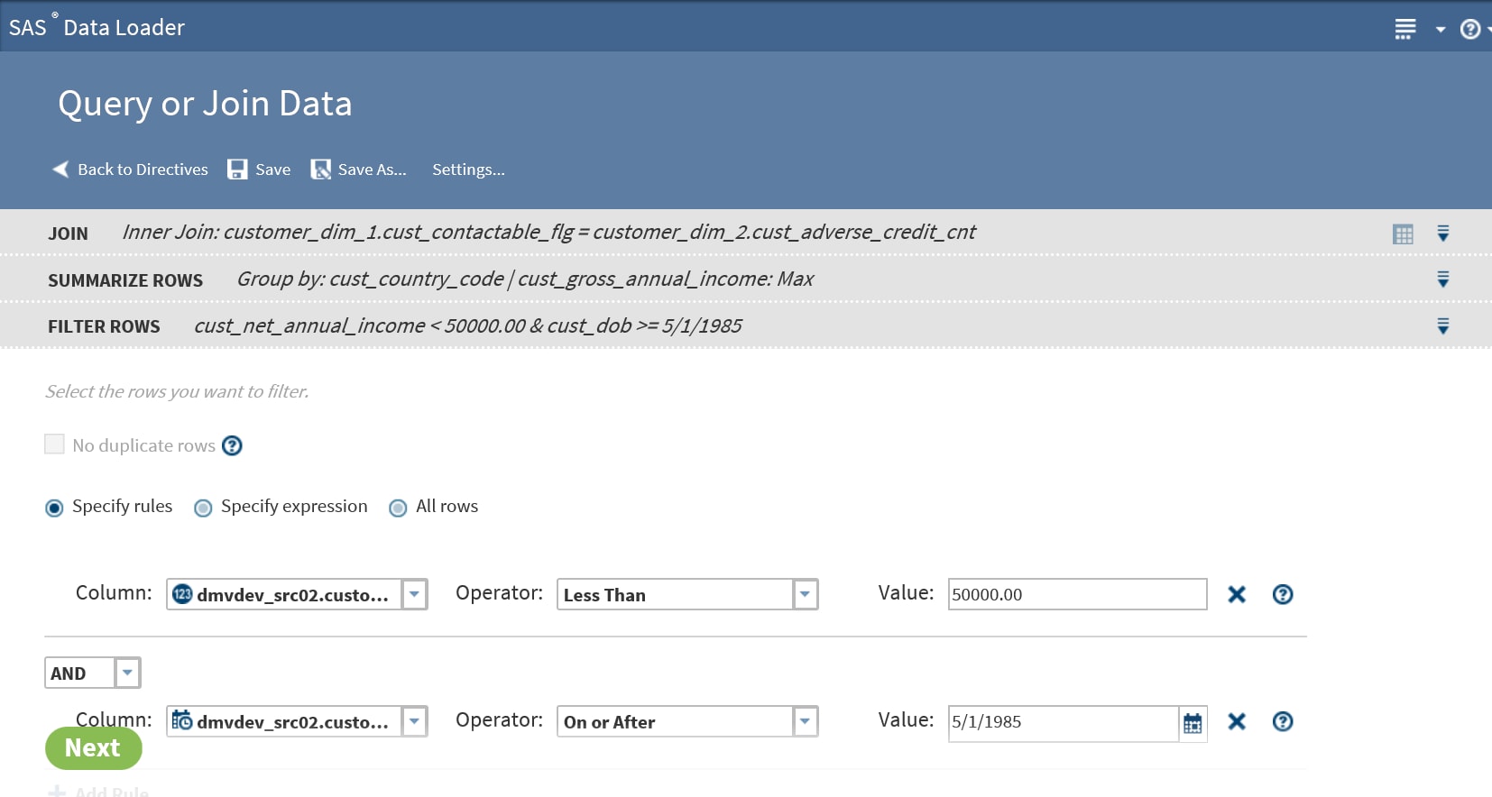
-
In the Value field, add the source column value that completes the expression. In the preceding example, the two rules combine to read “Filter from the target all source rows with an income less than 50,000.00 and born on or after May 1, 1985.”
-
Click Add Rule as needed to add another rule. Select a different column, operator, and value. To associate a new rule with the previous rules, either retain the default AND operator or click AND and select OR.
-
When your rules are complete, go to Step 27.
-
-
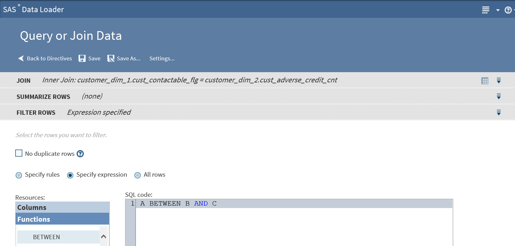
To filter rows using an expression, follow these steps:
-
In the expression text box, either enter or paste an expression.Your expression must use either HiveQL functions or Cloudera Impala SQL functions, depending on the selected SQL environment. Click Settings to display the selected SQL environment. To learn more about SQL environments, see Enable Support for Impala and Spark.To learn about the requirements for expressions, see Develop Expressions for Directives.
-
To add functions to your expression, click Functions in the Resources box, expand a category, select a function, and click
 .
.
-
To add column names to your expression, position the cursor in the expression text box, click Columns in the Resources box, click a source column, and then click.
-
-
When your rules or expression are complete, click Next to open the Columns task.
-
Use the Columns task to do the following:Note: The Columns task is available only if your job does not contain summaries. If your job does contain summaries, then click Next to display the Sort task.
-
Add all source columns to the target
 , add one source column to the target
  , remove one source column from the target
  (or
(or  ), and remove all source columns from the target
  .
.
-
Rename columns by clicking in the Target Name column.
-
Move column to first or full-left position
 , move column left one position
  , move column right one position
  , and move column to last or full-right position
  .
.
-
Add a new column that will be populated with the results of a user-written expression. Click the Add icon.
The expression must use either HiveQL or Cloudera Impala SQL. To see the selected SQL environment, click Settings. For more information about SQL environments, see Enable Support for Impala and Spark,To learn the requirements for expressions, see Develop Expressions for Directives.
-
Add a new column and open the Advanced Editor to develop an expression. Click
 .
.
-
Modify or replace the data in an existing column using data that is returned by a user-written expression. Click
 .
.
-
-
Follow these steps to specify a user-written expression:
-
Either add a new column or verify the name of the column to be modified In the Column name field.
-
Paste or enter SQL code into the expression column, or open the Advanced Editor to create an expression.
-
In the Advanced Editor, select functions and column names from the Resources box to create your expression.
-
-
Click Next to close the Column name task and open the Target Table task.
-
In the Target Table task, to learn about the contents of a table, click the table and click the Table Viewer icon
 .
.
-
To write your target data to an existing table, click that table and click Next. Any and all existing data will be replaced.
-
To save data to a new target table, click
 , enter a table name in the New Table window,
and click OK.
The names of tables must meet the naming conventions of SAS and Hive.
, enter a table name in the New Table window,
and click OK.
The names of tables must meet the naming conventions of SAS and Hive. -
To display your target data as a view, select
 . Saving as a view displays your target data in Sample
Data Viewer without saving the results to a table on disk.
When your target selection is complete, click Next to open the Code task
. Saving as a view displays your target data in Sample
Data Viewer without saving the results to a table on disk.
When your target selection is complete, click Next to open the Code task -
In the Code task, click Edit Code to edit the generated code. Click Reset Code to restore the original generated code. Click Next to open the Result task.Note: Edit your SQL code with care. The code in the editor is the exact code that will be executed by your job, regardless of previous selections. Also, code changes are not reflected in prior tasks, so code regeneration does not retain code edits.
-
In the Result task, you can review the previous tasks by clicking on the gray bars at the top of the window.
-
Click Save or Save As to save your job.
-
Click Start to execute your directive. To monitor the progress of your job, see the Run Status directive.
Copyright © SAS Institute Inc. All Rights Reserved.