Response Surface Designs

Fitting a Model

Return to the main design window. You can fit a model by clicking Fit. Select THCKNESS.

To choose the ANOVA method of significant effect selection, select Identify Select effects Automatic ANOVA. The only automatic selection methods available for the response surface fit are ANOVA and Stepwise.

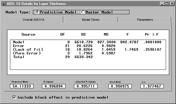
To display an ANOVA table, select Model Fit details. In the overall ANOVA window, you can review the fitted master model (the full model with all effects) or a smaller model that contains only the effects currently designated as significant in the master model. The overall ANOVA provides descriptive statistics for both models, including the response mean, root mean squared error (RMSE), R square, and the coefficient of variation. ADX will provide a lack-of-fit test whenever sufficient runs are available by splitting total error into pure error and error due to lack of fit. Since the -value for the lack of fit is large, the conclusion is that this model is adequate.

Close the window to return to the Effect Selection for Layer Thickness window.

Viewing Contour Plots from the Fit Window

ADX makes a contour plot accessible from the Effect Selection for Layer Thickness window. To view the plot, follow these steps:

1. Click the Contour Plot button to select the effects to use for generating the contour plot. You can choose to view the contour plot for the master model or the smaller model containing the selected effects.
   
   

   
   
   

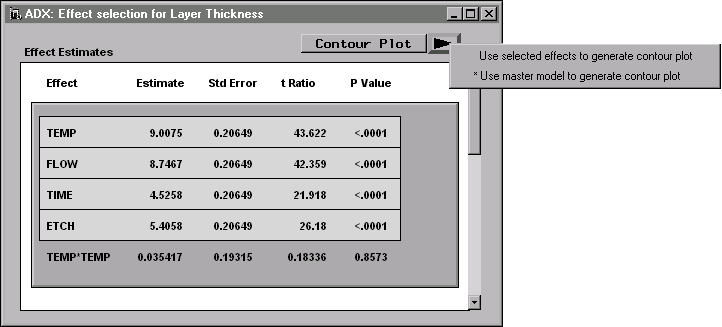
2. Click the arrow beside the Contour Plot button and select Use selected effects to generate contour plot.

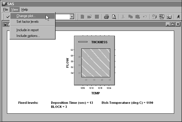
This is a contour plot showing how thickness varies with flow and deposition temperature for the fixed levels of the factors TIME, ETCH, and BLOCK shown at the bottom. The View menu enables you to modify the contour plots or include it in a report.

Select View Change plot to invoke the Contour Plot Wizard, which provides different options for viewing the contours.

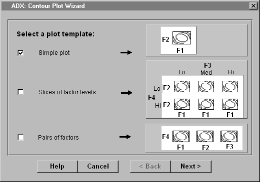
To view FLOW by TEMP contours at low, center, and high values of TIME for Block 2, follow these steps:

1. Select Slices of factor levels.
   
   

   
   
   

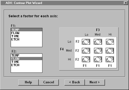
2. Select F1=TEMP and F2=FLOW from the two lists.
3. Click Next.
   
   

   
   
   

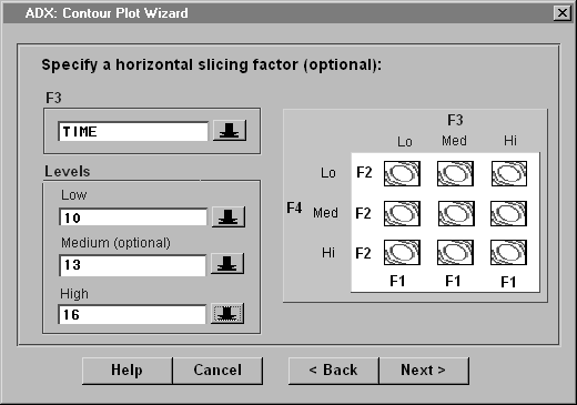
4. Select TIME as the horizontal slicing factor.
5. Use the arrows to change the levels for Low, Medium, and High to 7, 10, and 19, respectively.
6. Click Next to set factor levels for nondisplay variables.
   
   

   
   
   

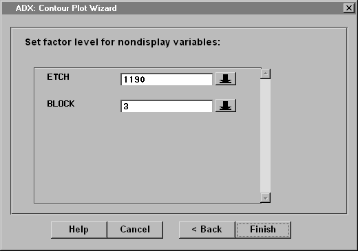
7. Click Finish. You should see the following display.
   
   

   
   
   

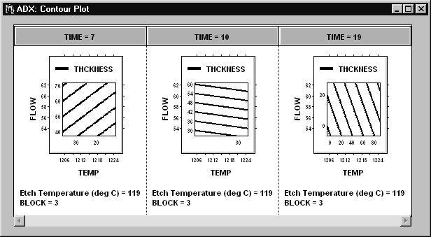
The small labels along the Y and X axes indicate the values of the contours of THCKNESS.

To create a FLOW by TEMP contour plot for THCKNESS at TIME=10, ETCH=1190, and BLOCK=1, click Change plot and follow the wizard steps.

To create a FLOW by TEMP contour plot for THCKNESS at TIME=10, ETCH=1190, and BLOCK=1, do the following:

1. Note that contour plots in ADX are highly interactive. Click on a contour line to grab and move contour lines.
2. Right-click to see the options available.
   
   

   
   
   

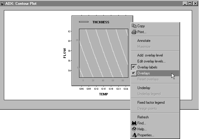
3. Select the Edit overlay levels option from the menu to open the Contour Levels window. You can use this window to select which fitted response to overlay, specify the grid, or have ADX generate automatic levels.
   
   

   
   
   

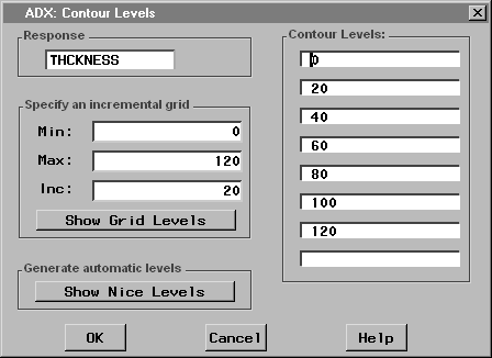
4. Click OK to close the Contour Levels window.

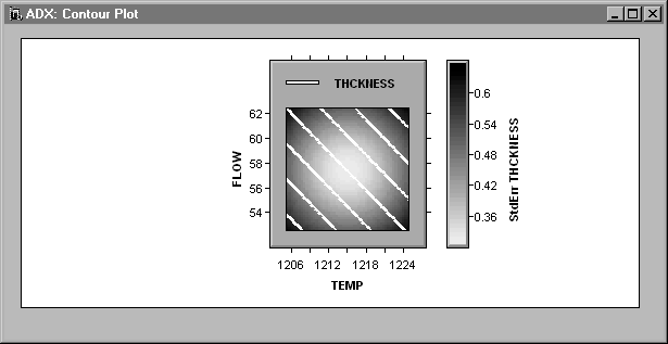
ADX can also display the standard error of the predicted response by using a shaded underlay. Right-click and select Underlay.

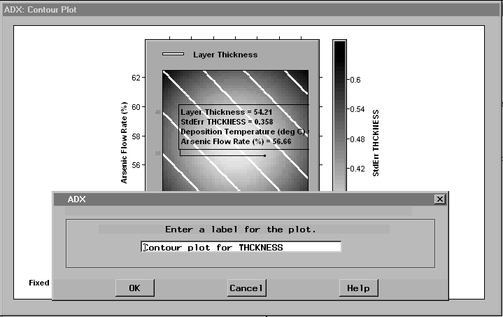
Press the left mouse button and move the mouse pointer over the plot to find those factor combinations that minimize the standard error (StdErr) and achieve a response close to the target of 60. As indicated by the thermometer legend, the lighter shade shows the factor region with the lowest standard error.

Annotating the Contour Plot

To annotate the contour plot with information about factor settings and to include the display in a report, do the following:

1. Right-click inside the contour plot.
2. Select Annotate to annotate the contour plot with the factor settings, response, and standard error of the response.
   
   

   
   
   

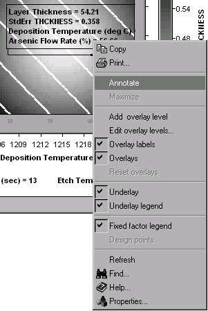
3. Move your mouse pointer within the contour plot to find the settings.
4. Click a point inside the plot to fix the annotation in place.

To remove the annotation, do the following:

1. Place your mouse pointer within the annotation box and right-click.
2. Select Annotate.

Canonical and Ridge Analyses

ADX performs canonical and ridge analyses for a response surface design when the master model contains all two-factor interactions and second-order polynomial terms, and when the design does not have more than one block. Refer to Myers and Montgomery (1995) for a description of canonical and ridge analyses.

The IC Fabrication design discussed in this chapter has three blocks, so is not a candidate for Canonical and Ridge analyses. The remainder of this section describes the analyses and displays the results for a design that does not have blocks.

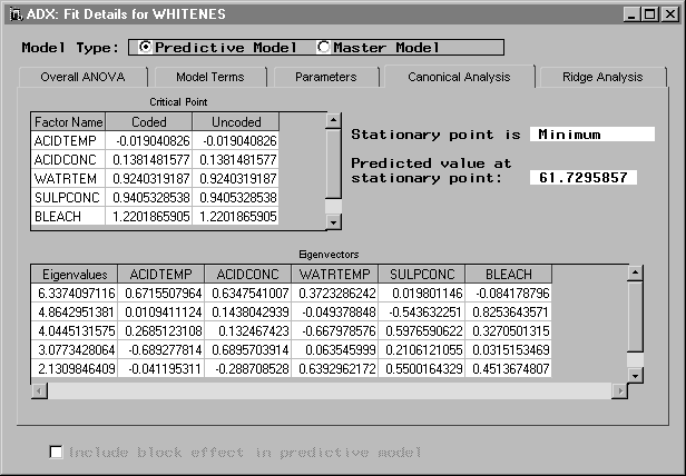
To request the canonical analysis, click Fit in the main design window and select Model Fit Details. If a canonical analysis is appropriate for a given design, then the Canonical Analysis and Ridge Analysis tabs will be displayed in the Fit Details window.

For the canonical analysis, ADX reports the coded and uncoded versions of the factor level settings for the critical (stationary) point and indicates the nature of the critical point (maximum, minimum, saddlepoint). It also reports the predicted response at the stationary point. Finally, it reports the eigenvectors and eigenvalues of the matrix of estimates of the second-order coefficients.

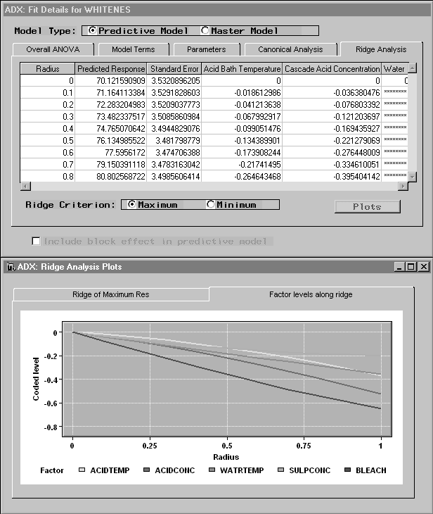
For the ridge analysis, ADX reports predicted values and factor settings along a ridge of optimum response, starting at the origin. Each point shows the factor settings that optimize---either minimize or maximize---the response at a given radius from the origin. A plot of the predicted response against the distance from the origin and a plot of the direction of the different responses along the axis can be requested by clicking Plots.