Full Factorial Designs

Optimizing Multiple Responses

ADX provides a variety of methods for determining which factor settings yield optimal values for one or more responses. One of these methods uses an interactive response profile plot, referred to as the prediction profiler, which you can augment with a desirability function for each response. For theoretical details, refer to Derringer and Suich (1980) and Montgomery (1997).

To find the optimal factor settings, do the following:

1. For each response you should have a predictive model. If not, ADX will use the master model for any response that does not have a predictive model.
2. Click Optimize in the main design window to open the Response Optimization window. Click Run to open the Prediction Profiler.
3. Review the Prediction Profiler settings.
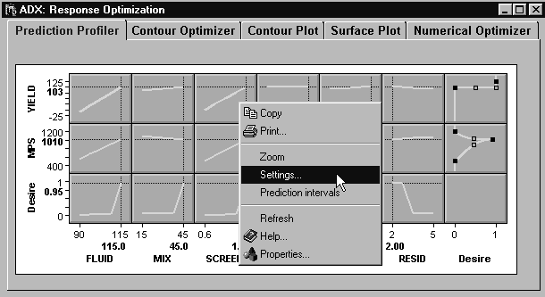
4. Review the interactive features by right-clicking in the Prediction Profiler.
5. View the desirability function.
6. Set the desirability function for each response so that high values of YIELD are desirable, and set a target of 1000 for MPS where values even moderately far away have very low desirability.
7. Review the factor settings that maximize the overall desirability, where the overall desirability function is the geometric mean of all the individual desirability functions.
8. Use the prediction calculator to determine the predicted responses along with their standard errors.

Optimizing Factor Settings

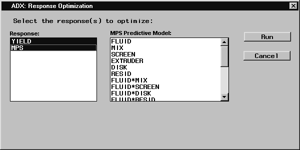
To get started, click Optimize. When you have multiple responses, ADX opens a window for you to select which responses to include in the optimization. Select both responses, YIELD and MPS. For each response ADX will remind you of the effects in the predictive model, as in the following illustration:

Click Run. ADX then displays the Prediction Profiler tab, which contains an interactive optimization tool that describes the change in responses as each factor is changed.

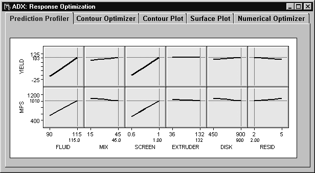
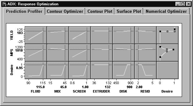
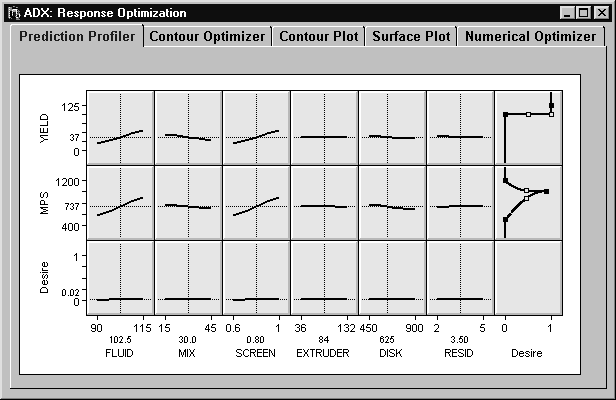
Interactive Prediction Profiler

The various components of the Prediction Profiler tab are as follows:

• The horizontal axis displays the factor names or labels with current settings indicated by vertical lines.
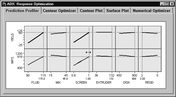
• The current setting for a factor can be changed by dragging the vertical line to the left or right.
• The vertical axis displays the predicted response for each response variable.
• The horizontal line is the predicted response for the current factor settings and will change as you change the factor settings.
• The plotted line in each plot is the prediction line for that response and that factor, assuming that all the other factors are held constant at the settings indicated by vertical lines.
• Prediction intervals can be toggled on or off by right-clicking and selecting Prediction intervals from the menu.

Simultaneous Optimization with Desirability Functions

The performance of a product or process frequently depends on whether the responses meet certain criteria. Here you want to maximize YIELD while holding MPS to a target value.

Alternatively, you specify a desirability function for each response that expresses its criterion. ADX computes an overall desirability as the geometric mean (the th root of the product of the individual desirability function, where is the number of responses). You can then change the factor settings to find values that maximize the overall desirability. Refer to Derringer and Suich (1980) and Montgomery (1997) for more details.

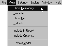
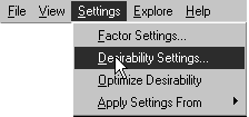
Select View Show Desirability.

ADX adds a desirability function for each response and an overall desirability trace for each factor.

The last column of cells is an interactive graph showing the desirability function for each response. The bottom row of cells displays the desirability trace corresponding to the settings of each factor.

The desirability function has three points that can be set: high, low, and center. These points take on values from 0 to 1, where 0 is least desirable and 1 is most desirable. By default, this function is linear and maximizes the response.

Since only very high values of YIELD are desirable, you need to reset the function. You can set the desirability function in two ways:

• indirectly, by changing the desirability settings in the Prediction Profiler Settings window
• directly, by clicking and dragging on the function line

To change the settings by using the Prediction Profiler Settings window, follow these steps:

1. Right-click and select Settings from the menu.
   
   

   
   
   

2. Click Desirability Setting.
3. The YIELD response should already be chosen; if not, click the down arrow and select it.
4. Select Any response in range.
5. Type 100 for the low limit. Keep the high limit setting.
   
   

   
   
   

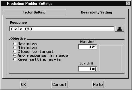
6. Click OK.

To change the settings by clicking and dragging, follow these steps:

1. Click and drag on the middle of the function line to the right so that the response has a desirability of 1 near 1000.
   
   

   
   
   

2. Click and drag the high and low ends of the function line to the left so that values not near 1000 have low desirability.
3. Since you want the desirability to decrease rapidly as the value moves away from 1000, drag the hollow lines to change the curvature of the desirability line.

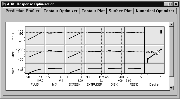
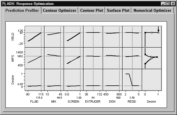
The result should look like the following figure:

The new desirability traces for each factor are given in the row at the bottom of the Prediction Profiler. The goal is to find factor settings that provide an overall desirability value close to 1. The individual factor desirability traces indicate how a factor will affect desirability. For example, shifting MPS away from 1000 decreases the desirability rapidly, and shifting YIELD to less than 100 results in a zero desirability.

At the factor setting where all factors are at their midpoint, the lack of slope for each factor indicates that desirability will be little affected by shifting any one factor. This is because the desirability is zero over a large interval of YIELD. However, the desirability traces are likely to change once factor settings are changed, especially since several significant interactions are identified. (Note that you might see slight differences between what is on your screen and what is shown here. The appearance of the traces depends on how the desirability functions are set.)

Shift FLUID, MIX, SCREEN, and DISK to their highest settings. The desirability trace for RESID changes dramatically.

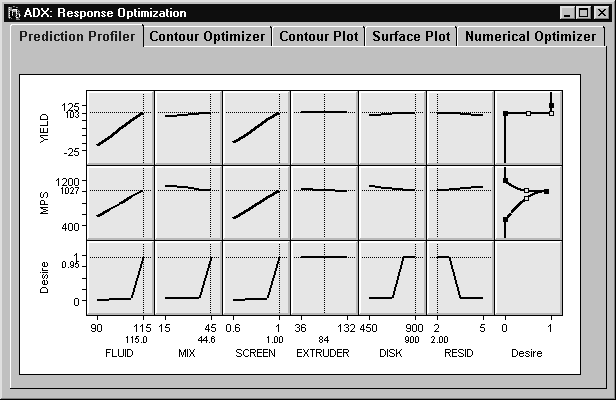
Shift RESID to its lowest settings. The desirability for this new setting is greater than 0.9. Note that the trace for EXTRUDER is flat; this indicates that you can set EXTRUDER according to other conditions without severely affecting your optimization.

You can also find the settings that maximize the desirability by selecting Optimize Desirability from the Settings menu. In this case, doing so with the preceding settings will only move EXTRUDER to its highest setting (this raises the desirability by a very small amount).

Once you have maximized desirability, you can review the individual factor traces to see how changing each factor changes the desirability, and in what direction.

Using the Optimization Results

There are several facilities you can use once you have identified the optimal factor settings:

1. Select View Include in Report and click OK to save the Prediction Profiler display in a report.
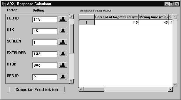
2. Select Explore Response calculator. The Response Calculator window will appear. Note that the factor settings are the same as those in the Prediction Profiler.
3. Click Compute Prediction. A row will be added to the spreadsheet. This row contains the factor settings, the predicted values for all responses, and the standard errors for all predictions within parentheses.
   
   

   
   
   

4. Close the window and click OK to return to the Response Optimization window.
5. Close the Response Optimization window and click Yes to return to the main design window.

You are now ready to report your results.