Full Factorial Designs

Fitting a Model

After exploring the data, you need to decide on a model you will use to predict or optimize the response. This model, referred to as the predictive model, will typically contain only effects that are considered to be significant.

When you first choose a design, ADX automatically defines a default master model to go with that design. Usually, the model includes an intercept, all main effects, and all two-factor interactions. Of course, you can choose a different master model. When you click Fit, ADX automatically fits the master model and highlights significant (active) effects in the Effect Selection for Yield () window. You can accept this list or refine it interactively by applying other automatic effect selection methods or by overriding the default effect selection. When you finish the effect selection process, ADX will retain the significant effects in a final model, which is called the predictive model.

You should create a predictive model before using Optimize, but if you do not, ADX will use the master model for optimization.

To fit the master model, follow these steps:

1. Click Fit in the main design window. Since this design has more than one response, a dialog box will appear to let you to choose a response.
   
   

   
   
   

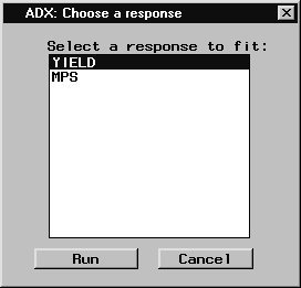
2. Select the YIELD response and click Run.
3. ADX will display a Check Fit Assumptions window. Since you want to analyze untransformed data for now, close this window.

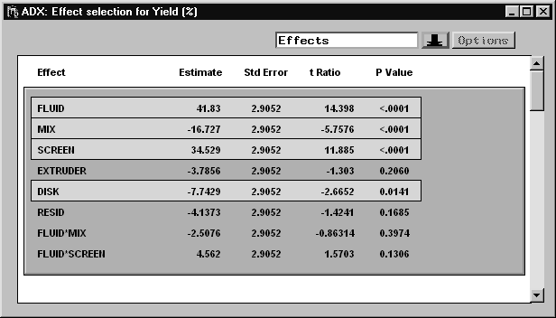
The Effect Selection for Yield () window displays the fitted master model and highlights the significant effects, which are determined by an automatic effect selection method. In this example, the master model includes all main effects and all two-factor interactions. Four of the main effects (highlighted) and a number of two-factor interactions (not shown) were found to be significant based on analysis of variance, which is the automatic effect selection method used by default.

ADX provides a variety of automatic selection methods to determine significant effects . Each of these methods is explained in the ADX Help.

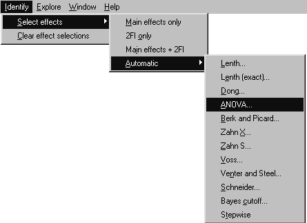
You can see the methods available for effect selection by selecting Identify Select effects Automatic.

When there are enough runs to form an independent estimate of the error variance, analysis of variance (ANOVA) is the default method used for determining the selected effects. When the design is saturated (insufficient runs to estimate an error variance), Lenth's (1989) method for selecting effects is used. See the section "Analyzing Saturated Designs" for more details on which effect selection methods are available for two-level designs.

Selecting ANOVA brings up the Parameters window, which enables you to change the alpha level used for effect selection. Note that other selection methods might have different parameters; the Parameters window will vary depending on the selection method you choose.

ADX highlights effects in the fitted model that are significant. By default, ADX selects the following significant effects:

• Main effects: FLUID, MIX, SCREEN, DISK
• Two-factor interactions: FLUID*DISK, MIX*SCREEN, SCREEN*DISK, SCREEN*RESID

ADX provides the ability to override selected effects. If you click on a highlighted effect to exclude it from the predictive model, ADX will consider it not to be significant, and the highlighting will disappear. If you click on an effect that is not highlighted, ADX will treat it as a significant effect, and it will be highlighted.

By default, ADX tests only two-way interactions. This is because the master model includes only intercept, main effects, and two-factor interactions. However, you might want to test for the presence of three-way interactions in this design. If so, you must change the master model. Follow these steps:

1. In the Effect Selection for Yield () window, select Model Change master model.
2. Select all the factors. This can be done by clicking FLUID and dragging down the list or by holding down the CTRL key and clicking on each factor.
3. In the edit box under the Interaction button, change the number to 3. You can click the right arrow button.
4. Click Interaction. All combinations of three-way interactions will be added to the Effects in Master Model list. ADX will now test for these effects.
5. Click OK. ADX might open the Check Fit Assumptions window and indicate that a response transform is necessary. For now, close this window without making any changes.
6. Scroll through the Effect Selection for Yield () window and notice the presence of three-way interactions. The FLUID*MIX*SCREEN effect is automatically selected, indicating that this effect is statistically significant at the level. This agrees with the assessment made previously with the -way interaction plot. ADX also selects FLUID*MIX*DISK, FLUID*SCREEN*DISK, FLUID*SCREEN*RESID, MIX*SCREEN*DISK, and MIX*SCREEN*RESID.

The effect selector is one of several displays you can use to display effects. Click the icon at the top to see a list of the different types of displays available for effect selection. Note that the selection of significant (active) effects is maintained from one display to another.

Normal Plot Display

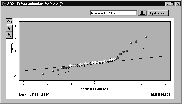
The normal plot is a common method for displaying significant effects in factorial designs.

To display the normal plot, click the down arrow and select Normal plot from the pop-up menu. ADX highlights significant effects (according to the ANOVA method of selection) by using large, round symbol markers.

Three different modes are available for interacting with this plot. Click on the corresponding icon to enter each mode:

Use the labeling mode to display the label for an effect by clicking on the point you want to label or remove the label from.

Use the selection mode to overwrite the selection of significant (active) effects by clicking on points you want to select or deselect. Significant (active) effects are highlighted.

Use the magnification mode to drag a rectangular area in the normal plot for magnification.

Note that two reference lines are displayed in the normal plot. These lines can be used for visual assessment of effects. Points that depart from the lines are considered to correspond with active effects.

Both lines pass through the origin. The slope of the dashed line is the root mean squared error (RMSE) calculated from ANOVA. This line is displayed only when an ANOVA can be performed. The slope of the solid line is Lenth's pseudostandard error (PSE) . You can display alternative PSE reference lines by clicking the Options button from the Normal Plot. ADX provides options for the horizontal axis scale and for computing the pseudostandard error.

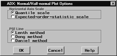
Select which options you want, and click OK to make the change.

Half-Normal Plot

Some experimenters prefer the half-normal plot over the normal plot. In a half-normal plot the magnitudes of the effects are displayed rather than the effects themselves.

To display the half-normal plot, click the down arrow and select Half-normal Plot from the pop-up menu.

You can use exactly the same methods for changing the options and selected effects that you use in the normal plot.

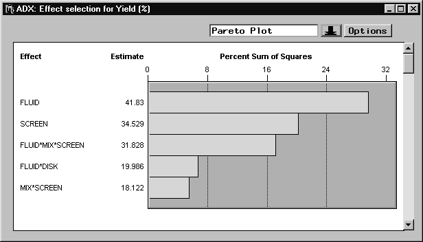
Pareto Plot

The Pareto plot displays effect estimates in decreasing order from largest to smallest. This makes it easy to determine the most important effects in the model. Pareto plot options can be used to change the type of estimate displayed from percent sum of squares to absolute effect.

To view the estimates with the Pareto plot display, click the down arrow and select Pareto Plot from the pop-up menu.