Time Series Exploration Task

Example: Exploring the SASHELP.PRICEDATA Data Set

About the Time Series Exploration Task

The Time Series Exploration task creates graphs and statistics that enable you to view and analyze your time series data.

Example: Exploring the SASHELP.PRICEDATA Data Set

To create this example:

In the Tasks section, expand the Forecasting folder and double-click Time Series Exploration. The user interface for the Time Series Exploration task opens.
On the Data tab, select the SASHELP.PRICEDATA data set.
Assign columns to these roles and specify these options:
1. To the Dependent variable role, assign the sale variable.
2. Expand the Additional Roles heading. To the Time ID role, assign the date variable. From the Interval drop-down list, select Quarter.
3. Under the Roles heading, locate the Transformations table. For the sale variable, find the Accumulation drop-down list, and select Sum as the accumulation method.
Click the Analyses tab, and select these series plots:
- Time Series
- Series histogram
- Seasonal cycles
To run the task, click .

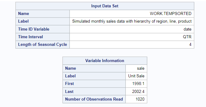
The first part of the results describes the input data set. This information shows the name and interval of the time ID variable and information about the dependent variable.

The time series plot suggests that there is a cyclical nature to sales for this product.

The histogram shows the distribution of sales for the series. Both a normal distribution and a kernel distribution are overlaid on the histogram.

The seasonal cycle plot shows that sales peak in Quarter 2 and are the lowest in Quarter 4.

Assigning Data to Roles

To run the Time Series Exploration task, you must assign a column to the Dependent variable role.

Role	Description
Roles
Dependent variable	specifies the dependent variable.
Independent variables	specifies any explanatory, input, predictor, or causal factor variables. You can assign only numeric variables to this role.
Transformations	specifies the transformations and simple differencing for the dependent and independent variables. If you assign a variable to the Time ID role, you can also specify an accumulation method. If the season length is greater than 1, you can specify seasonal differencing.
Additional Roles
Time ID	specifies the column that contains the time ID values.
Properties
Interval	specifies the interval for the time ID variable. For more information about SAS time intervals, see Understanding SAS Time Intervals.
Multiplier	specifies the multiplier for the time interval. By default, the multiplier is 1. This value cannot be negative.
Shift	specifies the shift for the time interval. By default, the shift is 1. This value cannot be negative.
Season length	specifies the seasonality of the time interval. The default value depends on the time interval.
Additional Roles
Season length	enables you to specify the seasonality of the data when you do not assign a time ID variable.
Group analysis by	lists the variable or variables that you want to use as the classification (BY) variables.

Setting the Analyses Options

Option Name	Description
Series Plots
You can include these series plots in your results: time series plot series histogram seasonal cycles
Statistics
You can include these statistics in your results: the descriptive statistics for the accumulated time series a table of the seasonal statistics the seasonal decomposition and adjustment table the trend statistics table
Autocorrelation Analysis
Perform autocorrelation analysis	specifies to include an autocorrelation analysis in the results.
Select plots to display	specifies the plots to display in the results. By default, the results show the autocorrelation analysis panel. However, you can select whether to include these plots in the results as well: autocorrelation function normalized autocorrelation function partial autocorrelation function normalized partial autocorrelation function inverse autocorrelation function normalized inverse autocorrelation function white noise probability test white noise probability test (log scale)
Number of lags	specifies the lag values. By default, the number of lags is 0.
Cross-Correlation Analysis Note: To perform a cross-correlation analysis, you must assign a variable to the Independent variables role.
Perform cross-correlation analysis	specifies to include a cross-correlation analysis in the results.
Plots	specifies the plots to include in the results. A cross-series plot is included by default. You can also include a cross-correlation function plot and a normalized cross-correlation function plot.
Decomposition Analysis Note: To perform a decomposition analysis, the seasonal cycle length must be greater than 1.
Perform decomposition analysis	specifies to include a decomposition analysis in the results.
Select plots to display	specifies the plots to include in the results. By default, the decomposition panel is included. You can choose to include these plots as well: a plot of the components a plot of the seasonally adjusted series a plot of the seasonally adjusted series (percent change)
Decomposition method	specifies the decomposition method to use when creating the selected decomposition analysis plots.
Spectral Density Analysis
Spectral density estimate plot	specifies whether to include a spectral density plot in the results.
Minimum period	specifies the minimum period to include in the spectral density plot. This value must be an integer greater than or equal to 0 and less than or equal to 32,767.
Details
Adjust the series by its mean prior to the analysis	specifies whether the series should be adjusted by its mean before performing the Fourier decomposition.
Analysis domain	specifies how the smoothing function is interpreted. You can choose from these options: Frequency smooths the periodogram ordinates. This is the default. Time applies the kernel as a filter to the time series autocovariance function.
Kernel Specifications
Kernel function	specifies the kernel function to use in the analysis. By default, no kernel function is specified. You can choose from these options: Parzen kernel Bartlett kernel Tukey-Hanning kernel Truncated kernel Quadratic spectral kernel
Scale coefficient	specifies the scale coefficient for the kernel function.
Exponent	specifies the exponent for the kernel function.
Unit Root Test Analysis
Perform augmented Dickey-Fuller test	specifies whether to perform an augmented Dickey-Fuller test.
Augmenting order	specifies the augmenting order for the Dickey-Fuller test. This value must be an integer greater than or equal to 0 and less than or equal to 1,000.