The TTEST Procedure

Comparing Group Means
If you want to compare values obtained from two different groups, and if the groups are independent of each other and the data are normally or lognormally distributed in each group, then a group t test can be used. Examples of such group comparisons include the following:
-
test scores for two third-grade classes, where one of the classes receives tutoring
-
fuel efficiency readings of two automobile nameplates, where each nameplate uses the same fuel
-
sunburn scores for two sunblock lotions, each applied to a different group of people
-
political attitude scores of males and females
In the following example, the golf scores for males and females in a physical education class are compared. The sample sizes from each population are equal, but this is not required for further analysis. The scores are thought to be approximately normally distributed within gender. The data are read by the following statements:
data scores;
   input Gender $ Score @@;
   datalines;
f 75  f 76  f 80  f 77  f 80  f 77  f 73
m 82  m 80  m 85  m 85  m 78  m 87  m 82
;
The dollar sign ($) following Gender in the INPUT statement indicates that Gender is a character variable. The trailing at signs (@@) enable the procedure to read more than one observation per line.
You can use a group t test to determine whether the mean golf score for the men in the class differs significantly from the mean score for the women. If you also suspect that the distributions of the golf scores of males and females have unequal variances, then you might want to specify the COCHRAN option in order to use the Cochran approximation (in addition to the Satterthwaite approximation, which is included by default). The following statements invoke PROC TTEST for the case of unequal variances, along with both types of confidence limits for the pooled standard deviation.
ods graphics on;

proc ttest cochran ci=equal umpu;
   class Gender;
   var Score;
run;

ods graphics off;
The CLASS
statement contains the variable that distinguishes the groups being compared, and the VAR
statement specifies the response variable to be used in calculations. The COCHRAN
option produces p-values for the unequal variance situation by using the Cochran and Cox (1950) approximation. Equal-tailed and uniformly most powerful unbiased (UMPU) confidence intervals for  are requested by the CI=
option. Output from these statements is displayed in Figure 119.4 through Figure 119.7.
are requested by the CI=
option. Output from these statements is displayed in Figure 119.4 through Figure 119.7.
Figure 119.4: Simple Statistics
Simple statistics for the two populations being compared, as well as for the difference of the means between the populations, are displayed in Figure 119.4. The Gender column indicates the population corresponding to the statistics in that row. The sample size (N), mean, standard deviation, standard error, and minimum and maximum values are displayed.
Confidence limits for means and standard deviations are shown in Figure 119.5.
Figure 119.5: Simple Statistics
| Gender | Method | Mean | 95% CL Mean | Std Dev | 95% CL Std Dev | 95% UMPU CL Std Dev | |||
|---|---|---|---|---|---|---|---|---|---|
| f | 76.8571 | 74.5036 | 79.2107 | 2.5448 | 1.6399 | 5.6039 | 1.5634 | 5.2219 | |
| m | 82.7143 | 79.8036 | 85.6249 | 3.1472 | 2.0280 | 6.9303 | 1.9335 | 6.4579 | |
| Diff (1-2) | Pooled | -5.8571 | -9.1902 | -2.5241 | 2.8619 | 2.0522 | 4.7242 | 2.0019 | 4.5727 |
| Diff (1-2) | Satterthwaite | -5.8571 | -9.2064 | -2.5078 | |||||
For the mean differences, both pooled (assuming equal variances for males and females) and Satterthwaite (assuming unequal variances) 95% intervals are shown. The confidence limits for the standard deviations are of the equal-tailed variety.
The test statistics, associated degrees of freedom, and p-values are displayed in Figure 119.6.
Figure 119.6: t Tests
The Method column denotes which t test is being used for that row, and the Variances column indicates what assumption about variances is being made. The pooled
test assumes that the two populations have equal variances and uses degrees of freedom  , where
  and
and  are the sample sizes for the two populations. The remaining two tests do not assume that the populations have equal variances.
The Satterthwaite test uses the Satterthwaite approximation for degrees of freedom, while the Cochran test uses the Cochran
and Cox approximation for the p-value. All three tests result in highly significant p-values, supporting the conclusion of a significant difference between males’ and females’ golf scores.
are the sample sizes for the two populations. The remaining two tests do not assume that the populations have equal variances.
The Satterthwaite test uses the Satterthwaite approximation for degrees of freedom, while the Cochran test uses the Cochran
and Cox approximation for the p-value. All three tests result in highly significant p-values, supporting the conclusion of a significant difference between males’ and females’ golf scores.
The "Equality of Variances" test in Figure 119.7 reveals insufficient evidence of unequal variances (the Folded F statistic  = 1.53, with p = 0.6189).
Figure 119.7: Tests of Equality of Variances
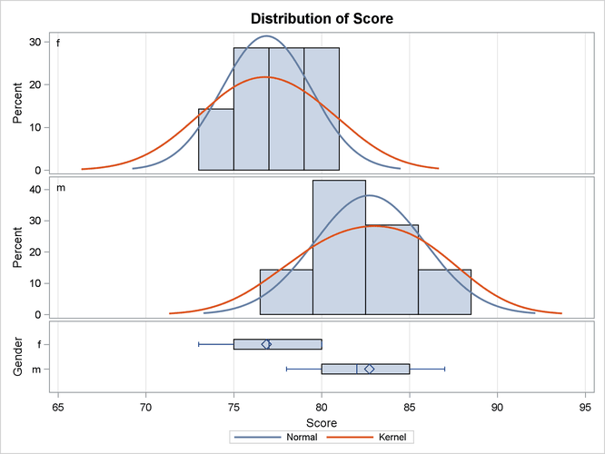
The summary panel in Figure 119.8 shows comparative histograms, normal and kernel densities, and box plots, comparing the distribution of golf scores between genders.
Figure 119.8: Summary Panel
The Q-Q plots in Figure 119.9 assess the normality assumption for each gender.
Figure 119.9: Q-Q Plot
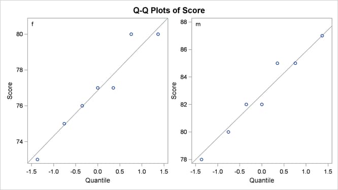
The plots for both males and females show no obvious deviations from normality. You can check the assumption of normality more rigorously by using PROC UNIVARIATE with the NORMAL option; if the assumption of normality is not reasonable, you should analyze the data with the nonparametric Wilcoxon rank sum test by using PROC NPAR1WAY.