The TTEST Procedure

One-Sample Design

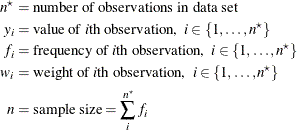
Define the following notation:

$\begin{align*} n^\star & = \mbox{number of observations in data set} \\ y_ i & = \mbox{value of }i\mbox{th observation,} \; \; i \in \{ 1, \ldots , n^\star \} \\ f_ i & = \mbox{frequency of }i\mbox{th observation,} \; \; i \in \{ 1, \ldots , n^\star \} \\ w_ i & = \mbox{weight of }i\mbox{th observation,} \; \; i \in \{ 1, \ldots , n^\star \} \\ n & = \mbox{sample size} = \sum _ i^{n^\star } f_ i \end{align*}$

Normal Data (DIST=NORMAL)

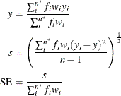
The mean estimate $\bar{y}$ , standard deviation estimate s, and standard error $\mr{SE}$ are computed as follows:

$\begin{align*} \bar{y} & = \frac{\sum _ i^{n^\star } f_ i w_ i y_ i}{\sum _ i^{n^\star } f_ i w_ i} \\ s & = \left( \frac{\sum _ i^{n^\star } f_ i w_ i (y_ i - \bar{y})^2}{n-1} \right)^\frac {1}{2} \\ \mr{SE} & = \frac{s}{\sum _ i^{n^\star } f_ i w_ i} \end{align*}$

The 100(1 – $\alpha$ )% confidence interval for the mean $\mu$ is

$\begin{align*} \left( \bar{y} - t_{1-\frac{\alpha }{2}, n-1} \mr{SE} \; \; , \; \; \bar{y} + t_{1-\frac{\alpha }{2}, n-1} \mr{SE} \right) & , \; \; \mbox{SIDES=2} \\ \left( -\infty \; \; , \; \; \bar{y} + t_{1-\alpha , n-1} \mr{SE} \right) & , \; \; \mbox{SIDES=L} \\ \left( \bar{y} - t_{1-\alpha , n-1} \mr{SE} \; \; , \; \; \infty \right) & , \; \; \mbox{SIDES=U} \end{align*}$

The t value for the test is computed as

$t = \frac{\bar{y} - \mu _0}{\mr{SE}}$

The p-value of the test is computed as

$p\mbox{-value} = \left\{ \begin{array}{ll} P \left( t^2 > F_{1-\alpha , 1, n-1} \right) \; \; , & \mbox{2-sided} \\ P \left( t < t_{\alpha , n-1} \right) \; \; , & \mbox{lower 1-sided} \\ P \left( t > t_{1-\alpha , n-1} \right) \; \; , & \mbox{upper 1-sided} \\ \end{array} \right.$

The equal-tailed confidence interval for the standard deviation (CI= EQUAL) is based on the acceptance region of the test of $H_0\colon \sigma =\sigma _0$ that places an equal amount of area ( $\frac{\alpha }{2}$ ) in each tail of the chi-square distribution:

$\left\{ \chi _{\frac{\alpha }{2},n-1}^{2} \leq \frac{(n-1)s^2}{\sigma _0^2} \leq \chi _{\frac{1-\alpha }{2},n-1}^{2} \right\}$

The acceptance region can be algebraically manipulated to give the following 100(1 – $\alpha$ )% confidence interval for $\sigma ^2$ :

$\left(\frac{(n-1)s^2}{\chi _{1-\frac{\alpha }{2},n-1}^2} \; \; , \; \; \frac{(n-1)s^2}{\chi _{\frac{\alpha }{2},n-1}^2}\right)$

Taking the square root of each side yields the 100(1 – $\alpha$ )% CI= EQUAL confidence interval for $\sigma$ :

$\left(\left(\frac{(n-1)s^2}{\chi _{1-\frac{\alpha }{2},n-1}^2}\right)^\frac {1}{2} \; \; , \; \; \left( \frac{(n-1)s^2}{\chi _{\frac{\alpha }{2},n-1}^2} \right)^\frac {1}{2} \right)$

The other confidence interval for the standard deviation (CI= UMPU) is derived from the uniformly most powerful unbiased test of $H_0\colon \sigma =\sigma _0$ (Lehmann 1986). This test has acceptance region

$\left\{ c_1 \leq \frac{(n-1)s^2}{\sigma _0^2} \leq c_2 \right\}$

where the critical values $c_1$ and $c_2$ satisfy

$\int _{c_1}^{c_2}f_{n-1} (y)dy=1-\alpha$

and

$\int _{c_1}^{c_2}yf_{n-1} (y)dy=(n-1)(1-\alpha )$

where $f_\nu (y)$ is the PDF of the chi-square distribution with $\nu$ degrees of freedom. This acceptance region can be algebraically manipulated to arrive at

$P\left\{ \frac{(n-1)s^2}{c_2} \leq \sigma ^2 \leq \frac{(n-1)s^2}{c_1} \right\} =1-\alpha$

where $c_1$ and $c_2$ solve the preceding two integrals. To find the area in each tail of the chi-square distribution to which these two critical values correspond, solve $c_1 = \chi _{1-\alpha _2,n-1}^2$ and $c_2=\chi _{\alpha _1,n-1}^2$ for $\alpha _1$ and $\alpha _2$ ; the resulting $\alpha _1$ and $\alpha _2$ sum to $\alpha$ . Hence, a 100(1 – $\alpha$ )% confidence interval for $\sigma ^2$ is given by

$\left(\frac{(n-1)s^2}{\chi _{1-\alpha _2,n-1}^2} \; \; , \; \; \frac{(n-1)s^2}{\chi _{\alpha _1,n-1}^2}\right)$

Taking the square root of each side yields the 100(1 – $\alpha$ )% CI= UMPU confidence interval for $\sigma$ :

$\left(\left( \frac{(n-1)s^2}{\chi _{1-\alpha _2,n-1}^2} \right)^\frac {1}{2} \; \; , \; \; \left(\frac{(n-1)s^2}{\chi _{\alpha _1,n-1}^2} \right)^\frac {1}{2} \right)$

Lognormal Data (DIST=LOGNORMAL)

The DIST= LOGNORMAL analysis is handled by log-transforming the data and null value, performing a DIST= NORMAL analysis, and then transforming the results back to the original scale. This simple technique is based on the properties of the lognormal distribution as discussed in Johnson, Kotz, and Balakrishnan (1994, Chapter 14).

Taking the natural logarithms of the observation values and the null value, define

$\begin{align*} z_ i & = \log (y_ i) \; \; , \; \; i \in \{ 1, \ldots , n^\star \} \\ \gamma _0 & = \log (\mu _0) \end{align*}$

First, a DIST= NORMAL analysis is performed on $\{ z_ i\}$ with the null value $\gamma _0$ , producing the mean estimate $\bar{z}$ , the standard deviation estimate $s_ z$ , a t value, and a p-value. The geometric mean estimate $\hat{\gamma }$ and the CV estimate $\widehat{CV}$ of the original lognormal data are computed as follows:

$\begin{align*} \hat{\gamma } & = \exp (\bar{z}) \\ \widehat{CV} & = \left( \exp (s_ z^2) - 1 \right)^\frac {1}{2} \end{align*}$

The t value and p-value remain the same. The confidence limits for the geometric mean and CV on the original lognormal scale are computed from the confidence limits for the arithmetic mean and standard deviation in the DIST= NORMAL analysis on the log-transformed data, in the same way that $\hat{\gamma }$ is derived from $\bar{z}$ and $\widehat{CV}$ is derived from $s_ z$ .