The SIMNORMAL Procedure

Conditional Simulation
For a conditional simulation, this distribution of
![\[ \bY = \left[ \begin{array}{c} Y_1\\ Y_2\\ \vdots \\ Y_ k \end{array} \right] \]](images/statug_simnorm0022.png)
must be conditioned on the values of the CONDITION variables. The relevant general result concerning conditional distributions
of multivariate normal random variables is the following. Let  , where
![\[ \bX = \left[ \begin{array}{c} \bX _1\\ \bX _2\\ \end{array} \right] \]](images/statug_simnorm0024.png)
![\[ \bmu = \left[ \begin{array}{c} \bmu _1\\ \bmu _2\\ \end{array} \right] \]](images/statug_simnorm0025.png)
![\[ \Sigma = \left( \begin{array}{cc} \bSigma _{11} & \bSigma _{12}\\ \bSigma _{21} & \bSigma _{22}\\ \end{array} \right) \]](images/statug_simnorm0026.png)
and where  is
is  ,
,  is
is  ,
,  is
is  ,
,  is
is  , and
, and  is
is  , with
  . The full vector
  has simply been partitioned into two subvectors,
  and
and  , and
, and  has been similarly partitioned into covariances and cross covariances.
With this notation, the distribution of conditioned on  is
is  , with
![\[ \tilde{\bmu }=\bmu _1+\bSigma _{12}\bSigma _{22}^{-1}(\mb{x}_2-\bmu _2) \]](images/statug_simnorm0044.png)
and
![\[ \tilde{\bSigma } = \bSigma _{11}-\bSigma _{12}\bSigma _{22}^{-1}\bSigma _{21} \]](images/statug_simnorm0045.png)
See Searle (1971, pp. 46–47) for details.
Using the SIMNORMAL procedure corresponds with the conditional simulation as follows. Let  be the VAR variables as before (k is the number of variables in the VAR list). Let the mean vector for
  be denoted by
  . Let the CONDITION variables be denoted by
  (where n is the number of variables in the COND list). Let the mean vector for
  be denoted by
  and the conditioning values be denoted by
![\[ \mb{c} = \left[ \begin{array}{c} c_1\\ c_2\\ \vdots \\ c_ n\\ \end{array} \right] \]](images/statug_simnorm0052.png)
Then stacking
![\[ \bX = \left[ \begin{array}{c} \bY \\ \bC \end{array} \right] \]](images/statug_simnorm0053.png)
the variance of is
![\[ \bV = \mr{Var}(\bX ) = \bSigma = \left( \begin{array}{cc} \bV _{11} & \bV _{12}\\ \bV _{21} & \bV _{22}\\ \end{array} \right) \]](images/statug_simnorm0054.png)
where  ,
, 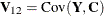 , and
, and  . By using the preceding general result, the relevant covariance matrix is
![\[ \tilde{\bV } = \bV _{11}-\bV _{12}\bV ^{-1}_{22}\bV _{21} \]](images/statug_simnorm0058.png)
and the mean is
![\[ \tilde{\bmu } = \bmu _1 + \bV _{12}\bV ^{-1}_{22}(\mb{c}-\bmu _2) \]](images/statug_simnorm0059.png)
By using  and
and  , simulating
 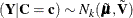 now proceeds as in the unconditional case.