The SEQDESIGN Procedure

Example 101.1 Creating Fixed-Sample Designs

This example demonstrates a one-sided fixed-sample design and a two-sided fixed-sample design. The following statements request a fixed-sample design with an upper alternative:

ods graphics on;
proc seqdesign pss
               ;
   OneSidedFixedSample: design nstages=1
                               alt=upper
                               alpha=0.025 beta=0.10
                               ;
   samplesize model=onesamplemean(mean=0.25);
run;

In the DESIGN statement, the label OneSidedFixedSample identifies the design in the output tables. The NSTAGES=1 option specifies that the design has only one stage; this corresponds to a fixed-sample design. In the SEQDESIGN procedure, the null hypothesis for the design is $H_0: \theta = 0$ and the ALT=UPPER option specifies an upper alternative hypothesis $H_1: \theta = \theta _1 > 0$ . The MEAN=0.25 option in the SAMPLESIZE statement specifies the upper alternative reference $\theta _1= 0.25$ .

The options ALPHA=0.025 and BETA=0.10 specify the Type I error probability level $\alpha = 0.025$ and the Type II error probability level $\beta = 0.10$ . That is, the design has a power $1-\beta = 0.90$ at $\theta _1= 0.25$ .

The "Design Information" table in Output 101.1.1 displays design specifications and the derived statistics such as power. As expected, the derived statistics such as maximum information and average sample number (in percentage of its corresponding fixed-sample information) are 100 for the fixed-sample design (NSTAGES=1). Also, for a fixed-sample design, the STOP= and METHOD= options in the DESIGN statement are not applicable.

Output 101.1.1: One-Sided Fixed-Sample Design Information

The SEQDESIGN Procedure

Design: OneSidedFixedSample

Design Information
Statistic Distribution	Normal
Boundary Scale	Standardized Z
Alternative Hypothesis	Upper
Alternative Reference	0.25
Number of Stages	1
Alpha	0.025
Beta	0.1
Power	0.9
Max Information (Percent of Fixed Sample)	100
Max Information	168.1188
Null Ref ASN (Percent of Fixed Sample)	100
Alt Ref ASN (Percent of Fixed Sample)	100

The "Method Information" table in Output 101.1.2 displays the $\alpha$ and $\beta$ error levels. It also displays the derived drift parameter, which is the standardized reference improvement, $\theta _{1} \sqrt {I_{0}}$ , where $\theta _{1}$ is the alternative reference and $I_{0}$ is the maximum information for the design. If either $\theta _{1}$ or $I_{0}$ is specified, the other statistic is derived in the SEQDESIGN procedure. For a fixed-sample design,

$\theta _{1} \sqrt {I_{0}} = \Phi ^{-1} (1-\alpha ) + \Phi ^{-1} (1-\beta ) = \Phi ^{-1} (0.975) + \Phi ^{-1} (0.90) = 3.2415$

Output 101.1.2: Method Information

Method Information
Boundary	Alpha	Beta	Alternative Reference	Drift
Upper Alpha	0.02500	0.10000	0.25	3.241516

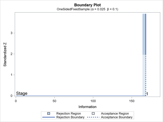
The "Boundary Information" table in Output 101.1.3 displays information level, alternative reference, and boundary value at each stage. The information proportion indicates the proportion of maximum information available at the stage. With only one stage for a fixed-sample design, the proportion is 1. With the SAMPLESIZE statement, the required sample size N is also displayed under the heading "Information Level."

Output 101.1.3: Boundary Information

Boundary Information (Standardized Z Scale) Null Reference = 0
_Stage_				Alternative	Boundary Values
	Information Level			Reference	Upper
	Proportion	Actual	N	Upper	Alpha
1	1.0000	168.1188	168.1188	3.24152	1.95996

By default (or equivalently if you specify BOUNDARYSCALE=STDZ), output alternative references and boundaries are displayed with the standardized normal Z scale. The alternative reference on the standardized Z scale at stage 1 is given by $\theta _1 \sqrt {I_1}$ , where $I_1$ is the information level at stage 1. With a boundary value 1.96, the hypothesis of $\theta = 0$ is rejected if the standardized normal statistic $Z \geq 1.96$ .

With ODS Graphics enabled, a detailed boundary plot with the rejection and acceptance regions is displayed, as shown in Output 101.1.4. The boundary values in the "Boundary Information" table in Output 101.1.3 are displayed in the plot.

Output 101.1.4: Boundary Plot

The "Sample Size Summary" table in Output 101.1.5 displays parameters for the sample size computation of the test for a normal mean.

Output 101.1.5: Sample Size Summary

Sample Size Summary
Test	One-Sample Mean
Mean	0.25
Standard Deviation	1
Max Sample Size	168.1188
Expected Sample Size (Null Ref)	168.1188
Expected Sample Size (Alt Ref)	168.1188

The "Sample Sizes (N)" table in Output 101.1.6 displays the derived sample sizes, in both fractional and integer numbers. With the resulting integer sample sizes, the corresponding information level is slightly larger than the level from the design. This can increase the power slightly if the integer sample size is used in the trial.

Output 101.1.6: Derived Sample Sizes

Sample Sizes (N) One-Sample Z Test for Mean
_Stage_	Fractional N		Ceiling N
_Stage_	N	Information	N	Information
1	168.12	168.1	169	169.0

The following statements request a two-sided fixed-sample design with a specified alternative reference:

ods graphics on;
proc seqdesign altref=1.2
               pss
               ;
   TwoSidedFixedSample: design nstages=1
                               alt=twosided
                               alpha=0.05 beta=0.10
                               ;
   samplesize model=twosamplemean(stddev=2 weight=2);
run;

In the SEQDESIGN procedure, the null hypothesis for the design is $H_{0}: \theta = 0$ . The ALT=TWOSIDED option specifies a two-sided alternative hypothesis $H_1: \theta = \theta _1 \neq 0$ . The ALTREF=1.2 option in the PROC SEQDESIGN statement specifies the alternative reference $\theta _1= \pm 1.2$ .

The ALPHA=0.05 option (which is the default) specifies the two-sided Type I error probability level $\alpha =0.05$ . That is, the lower and upper Type I error probabilities $\alpha _{l}=\alpha _{u}=0.025$ . The BETA=0.10 option (which is the default) specifies the Type II error probability level $\beta = 0.10$ , and the design has a power $1-\beta = 0.90$ at the alternative reference $\theta _1= \pm 1.2$ .

The "Design Information" table in Output 101.1.7 displays design specifications and the derived power. With a specified alternative reference, the maximum information is derived.

Output 101.1.7: Two-Sided Fixed-Sample Design Information

The SEQDESIGN Procedure

Design: TwoSidedFixedSample

Design Information
Statistic Distribution	Normal
Boundary Scale	Standardized Z
Alternative Hypothesis	Two-Sided
Alternative Reference	1.2
Number of Stages	1
Alpha	0.05
Beta	0.1
Power	0.9
Max Information (Percent of Fixed Sample)	100
Max Information	7.296822
Null Ref ASN (Percent of Fixed Sample)	100
Alt Ref ASN (Percent of Fixed Sample)	100

The "Method Information" table in Output 101.1.8 displays the $\alpha$ and $\beta$ errors, alternative references, and drift parameter. For a fixed-sample design, the derived drift parameter

$\theta _{1} \sqrt {I_{0}} = \Phi ^{-1}(1-\frac{\alpha }{2}) + \Phi ^{-1} (1-\beta ) = \Phi ^{-1} (0.975) + \Phi ^{-1} (0.90) = 3.2415$

Output 101.1.8: Method Information

Method Information
Boundary	Alpha	Beta	Alternative Reference	Drift
Upper Alpha	0.02500	0.10000	1.2	3.241516
Lower Alpha	0.02500	0.10000	-1.2	-3.24152

With a specified alternative reference $\theta _{1}= 1.2$ , the maximum information

$I_{0} = \left( \frac{3.2415}{1.2} \right)^{2} = 7.2968$

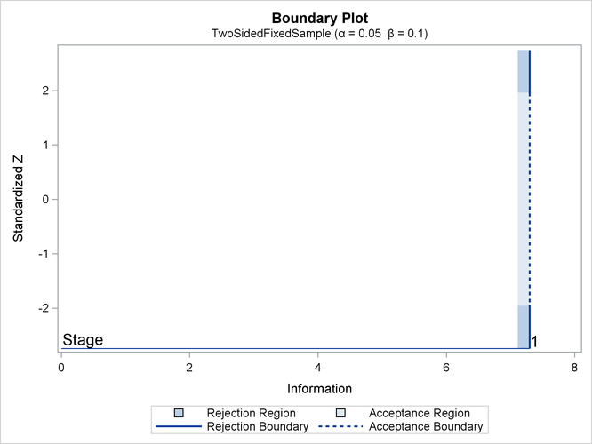
The default "Boundary Information" table in Output 101.1.9 displays information level, alternative reference, and boundary values. By default (or equivalently if you specify BOUNDARYSCALE=STDZ), the alternative reference and boundary values are displayed with the standardized normal Z scale. Thus, the standardized alternative references $\pm \theta _{1} \sqrt {I_{0}}$ are displayed.

Output 101.1.9: Boundary Information

Boundary Information (Standardized Z Scale) Null Reference = 0
_Stage_				Alternative		Boundary Values
	Information Level			Reference		Lower	Upper
	Proportion	Actual	N	Lower	Upper	Alpha	Alpha
1	1.0000	7.296822	131.3428	-3.24152	3.24152	-1.95996	1.95996

With boundary values of –1.96 and 1.96, the hypothesis of $\theta = 0$ is rejected if the standardized normal statistic $Z \geq 1.96$ or $Z \leq -1.96$ .

With ODS Graphics enabled, a detailed boundary plot with the rejection and acceptance regions is displayed, as shown in Output 101.1.10 . The boundary values in the "Boundary Information" table in Output 101.1.9 are displayed in the plot.

Output 101.1.10: Boundary Plot

The "Sample Size Summary" table in Output 101.1.11 displays parameters for the sample size computation of the test for a normal mean.

Output 101.1.11: Sample Size Summary

Sample Size Summary
Test	Two-Sample Means
Mean Difference	1.2
Standard Deviation	2
Max Sample Size	131.3428
Expected Sample Size (Null Ref)	131.3428
Expected Sample Size (Alt Ref)	131.3428
Weight (Group A)	2
Weight (Group B)	1

The "Sample Sizes (N)" table in Output 101.1.12 displays the derived sample sizes, in both fractional and integer numbers. With the WEIGHT=2 option, the allocation ratio is 2 for the first group and 1 for the second group. With the resulting integer sample sizes, the corresponding information level is slightly larger than the level from the design. This can increase the power slightly if the integer sample size is used in the trial.

Output 101.1.12: Derived Sample Sizes

Sample Sizes (N) Two-Sample Z Test for Mean Difference
_Stage_	Fractional N				Ceiling N
_Stage_	N	N(Grp 1)	N(Grp 2)	Information	N	N(Grp 1)	N(Grp 2)	Information
1	131.34	87.56	43.78	7.2968	132	88	44	7.3333