The RSREG Procedure

Example 99.1 A Saddle Surface Response Using Ridge Analysis
Myers (1976) analyzes an experiment reported by Frankel (1961) aimed at maximizing the yield of mercaptobenzothiazole (MBT) by varying processing time and temperature. Myers (1976) uses a two-factor model in which the estimated surface does not have a unique optimum. A ridge analysis is used to determine the region in which the optimum lies. The objective is to find the settings of time and temperature in the processing of a chemical that maximize the yield. The following statements produce Output 99.1.1 through Output 99.1.5:
data d;
   input Time Temp MBT;
   label Time = "Reaction Time (Hours)"
         Temp = "Temperature (Degrees Centigrade)"
         MBT  = "Percent Yield Mercaptobenzothiazole";
   datalines;
 4.0   250   83.8
20.0   250   81.7
12.0   250   82.4
12.0   250   82.9
12.0   220   84.7
12.0   280   57.9
12.0   250   81.2
 6.3   229   81.3
 6.3   271   83.1
17.7   229   85.3
17.7   271   72.7
 4.0   250   82.0
;
ods graphics on;
proc rsreg data=d plots=(ridge surface);
   model MBT=Time Temp / lackfit;
   ridge max;
run;
ods graphics off;
Output 99.1.1 displays the coding coefficients for the transformation of the independent variables to lie between –1 and 1 and some simple statistics for the response variable.
Output 99.1.1: Coding and Response Variable Information
Output 99.1.2 shows that the lack of fit for the model is highly significant. Since the quadratic model does not fit the data very well,
firm statements about the underlying process should not be based only on the current analysis. Note from the analysis of variance
for the model that the test for the time factor is not significant. If further experimentation is undertaken, it might be
best to fix Time at a moderate to high value and to concentrate on the effect of temperature. In the actual experiment discussed here, extra
runs were made that confirmed the results of the following analysis.
Output 99.1.2: Analyses of Variance
| Parameter | DF | Estimate | Standard Error |
t Value | Pr > |t| | Parameter Estimate from Coded Data |
|---|---|---|---|---|---|---|
| Intercept | 1 | -545.867976 | 277.145373 | -1.97 | 0.0964 | 82.173110 |
| Time | 1 | 6.872863 | 5.004928 | 1.37 | 0.2188 | -1.014287 |
| Temp | 1 | 4.989743 | 2.165839 | 2.30 | 0.0608 | -8.676768 |
| Time*Time | 1 | 0.021631 | 0.056784 | 0.38 | 0.7164 | 1.384394 |
| Temp*Time | 1 | -0.030075 | 0.019281 | -1.56 | 0.1698 | -7.218045 |
| Temp*Temp | 1 | -0.009836 | 0.004304 | -2.29 | 0.0623 | -8.852519 |
The canonical analysis (Output 99.1.3) indicates that the predicted response surface is shaped like a saddle. The eigenvalue of 2.5 shows that the valley orientation
of the saddle is less curved than the hill orientation, with an eigenvalue of –9.99. The coefficients of the associated eigenvectors
show that the valley is more aligned with Time and the hill with Temp. Because the canonical analysis resulted in a saddle point, the estimated surface does not have a unique optimum.
Output 99.1.3: Canonical Analysis
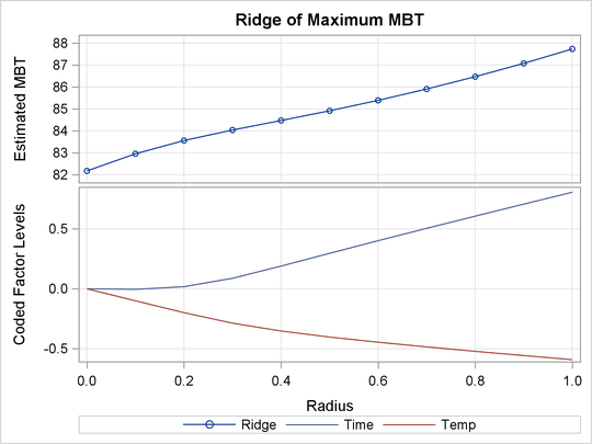
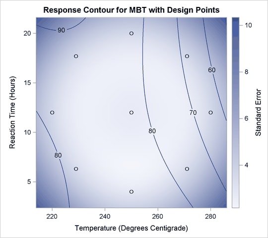
However, the ridge analysis in Output 99.1.4 and the ridge plot in Output 99.1.5 indicate that maximum yields result from relatively high reaction times and low temperatures. A contour plot of the predicted response surface, shown in Output 99.1.5, confirms this conclusion.
Output 99.1.4: Ridge Analysis
| Estimated Ridge of Maximum Response for Variable MBT: Percent Yield Mercaptobenzothiazole | ||||
|---|---|---|---|---|
| Coded Radius | Estimated Response | Standard Error |
Uncoded Factor Values | |
| Time | Temp | |||
| 0.0 | 82.173110 | 2.665023 | 12.000000 | 250.000000 |
| 0.1 | 82.952909 | 2.648671 | 11.964493 | 247.002956 |
| 0.2 | 83.558260 | 2.602270 | 12.142790 | 244.023941 |
| 0.3 | 84.037098 | 2.533296 | 12.704153 | 241.396084 |
| 0.4 | 84.470454 | 2.457836 | 13.517555 | 239.435227 |
| 0.5 | 84.914099 | 2.404616 | 14.370977 | 237.919138 |
| 0.6 | 85.390012 | 2.410981 | 15.212247 | 236.624811 |
| 0.7 | 85.906767 | 2.516619 | 16.037822 | 235.449230 |
| 0.8 | 86.468277 | 2.752355 | 16.850813 | 234.344204 |
| 0.9 | 87.076587 | 3.130961 | 17.654321 | 233.284652 |
| 1.0 | 87.732874 | 3.648568 | 18.450682 | 232.256238 |
Output 99.1.5: Ridge and Contour Plot of Predicted Response Surface