The PRINQUAL Procedure
- Overview
- Getting Started
-
Syntax

-
DetailsThe Three Methods of Variable TransformationUnderstanding How PROC PRINQUAL WorksSplinesMissing ValuesControlling the Number of IterationsPerforming a Principal Component Analysis of Transformed DataUsing the MAC MethodOutput Data SetAvoiding Constant TransformationsConstant VariablesCharacter OPSCORE VariablesREITERATE Option UsagePassive ObservationsComputational ResourcesDisplayed OutputODS Table NamesODS Graphics
-
Examples
- References
Example 92.1 Multidimensional Preference Analysis of Automobile Data
This example uses PROC PRINQUAL to perform a nonmetric multidimensional preference (MDPREF) analysis (Carroll 1972). MDPREF analysis is a principal component analysis of a data matrix with columns that correspond to people and rows that correspond to objects. The data are ratings or rankings of each person’s preference for each object. The data are the transpose of the usual multivariate data matrix. (In other words, the columns are people; in the more typical matrix the rows represent people.) The final result of an MDPREF analysis is a biplot (Gabriel 1981) of the resulting preference space. A biplot displays the judges and objects in a single plot by projecting them onto the plane in the transformed variable space that accounts for the most variance.
In 1980, 25 judges gave their preferences for each of 17 new automobiles. The ratings were made on a 0 to 9 scale, with 0 meaning very weak preference and 9 meaning very strong preference for the automobile. The following statements create a SAS data set with the manufacturer and model of each automobile along with the ratings:
title 'Preference Ratings for Automobiles Manufactured in 1980';

options validvarname=any;

data CarPref;
   input Make $ 1-10 Model $ 12-22 @25 ('1'n-'25'n) (1.);
   datalines;
Cadillac   Eldorado     8007990491240508971093809
Chevrolet  Chevette     0051200423451043003515698
Chevrolet  Citation     4053305814161643544747795
Chevrolet  Malibu       6027400723121345545668658
Ford       Fairmont     2024006715021443530648655
Ford       Mustang      5007197705021101850657555
Ford       Pinto        0021000303030201500514078
Honda      Accord       5956897609699952998975078
Honda      Civic        4836709507488852567765075
Lincoln    Continental  7008990592230409962091909
Plymouth   Gran Fury    7006000434101107333458708
Plymouth   Horizon      3005005635461302444675655
Plymouth   Volare       4005003614021602754476555
Pontiac    Firebird     0107895613201206958265907
Volkswagen Dasher       4858696508877795377895000
Volkswagen Rabbit       4858509709695795487885000
Volvo      DL           9989998909999987989919000
;
The following statements run PROC PRINCOMP and create a scree plot. The results of this step are shown in Output 92.1.1.
ods graphics on;
* Principal Component Analysis of the Original Data;
proc princomp data=CarPref;
   ods select ScreePlot;
   var '1'n-'25'n;
run;
Output 92.1.1: Eigenvalue Plot
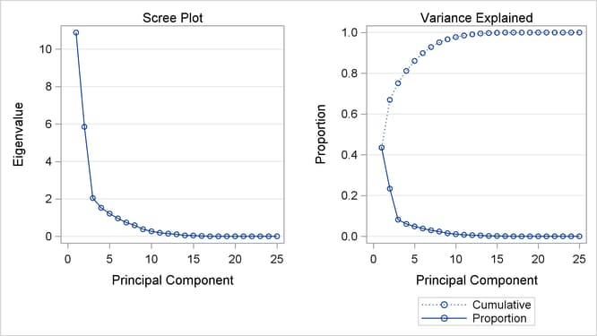
The scree or eigenvalue plot in Output 92.1.1 shows that two principal components should be retained. There is a clear separation between the first two components and the remaining components. There are eight eigenvalues that are precisely zero because there are eight fewer observations than variables in the data matrix. One additional eigenvalue is zero, for a total of nine zero eigenvalues, since the correlation matrix is based on centered data. The following statements create the data set and perform a principal component analysis of the original data.
PROC PRINQUAL fits the nonmetric MDPREF model. PROC PRINQUAL monotonically transforms the raw judgments to maximize the proportion
of variance accounted for by the first two principal components. The MONOTONE option is specified in the TRANSFORM statement
to request a nonmetric MDPREF analysis; alternatively, you can instead specify the IDENTITY option for a metric analysis.
Several options are used in the PROC PRINQUAL statement. The option DATA=CarPref specifies the input data set, OUT=Results creates an output data set, and N=2 and the default METHOD=MTV transform the data to better fit a two-component model. The
REPLACE option replaces the original data with the monotonically transformed data in the OUT= data set. The MDPREF option
standardizes the component scores to variance one so that the geometry of the biplot is correct, and it creates two variables
in the OUT= data set named Prin1 and Prin2. These variables contain the standardized principal component scores and structure matrix, which are used to make the biplot.
If the variables in data matrix  are standardized to mean zero and variance one, and n is the number of rows in , then
  is the principal component model, where
 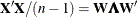 . The
. The  and
and  contain the eigenvectors and eigenvalues of the correlation matrix of . The first two columns of
  , the standardized component scores, and
  , which is the structure matrix, are output. The advantage of creating a biplot based on principal components is that coordinates
do not depend on the sample size. The following statements transform the data and produce Output 92.1.2.
, which is the structure matrix, are output. The advantage of creating a biplot based on principal components is that coordinates
do not depend on the sample size. The following statements transform the data and produce Output 92.1.2.
* Transform the Data to Better Fit a Two Component Model;
proc prinqual data=CarPref out=Results n=2 replace mdpref;
   title2 'Multidimensional Preference (MDPREF) Analysis';
   title3 'Optimal Monotonic Transformation of Preference Data';
   id model;
   transform monotone('1'n-'25'n);
run;
Output 92.1.2: PRINQUAL Iteration History
| Preference Ratings for Automobiles Manufactured in 1980 |
| Multidimensional Preference (MDPREF) Analysis |
| Optimal Monotonic Transformation of Preference Data |
| PRINQUAL MTV Algorithm Iteration History | |||||
|---|---|---|---|---|---|
| Iteration Number |
Average Change |
Maximum Change |
Proportion of Variance |
Criterion Change |
Note |
| 1 | 0.24994 | 1.28017 | 0.66946 | ||
| 2 | 0.07223 | 0.36958 | 0.80194 | 0.13249 | |
| 3 | 0.04522 | 0.29026 | 0.81598 | 0.01404 | |
| 4 | 0.03096 | 0.25213 | 0.82178 | 0.00580 | |
| 5 | 0.02182 | 0.23045 | 0.82493 | 0.00315 | |
| 6 | 0.01602 | 0.19017 | 0.82680 | 0.00187 | |
| 7 | 0.01219 | 0.14748 | 0.82793 | 0.00113 | |
| 8 | 0.00953 | 0.11031 | 0.82861 | 0.00068 | |
| 9 | 0.00737 | 0.06461 | 0.82904 | 0.00043 | |
| 10 | 0.00556 | 0.04469 | 0.82930 | 0.00026 | |
| 11 | 0.00445 | 0.04087 | 0.82944 | 0.00014 | |
| 12 | 0.00381 | 0.03706 | 0.82955 | 0.00011 | |
| 13 | 0.00319 | 0.03348 | 0.82965 | 0.00009 | |
| 14 | 0.00255 | 0.02999 | 0.82971 | 0.00006 | |
| 15 | 0.00213 | 0.02824 | 0.82976 | 0.00005 | |
| 16 | 0.00183 | 0.02646 | 0.82980 | 0.00004 | |
| 17 | 0.00159 | 0.02472 | 0.82983 | 0.00003 | |
| 18 | 0.00139 | 0.02305 | 0.82985 | 0.00003 | |
| 19 | 0.00123 | 0.02145 | 0.82988 | 0.00002 | |
| 20 | 0.00109 | 0.01993 | 0.82989 | 0.00002 | |
| 21 | 0.00096 | 0.01850 | 0.82991 | 0.00001 | |
| 22 | 0.00086 | 0.01715 | 0.82992 | 0.00001 | |
| 23 | 0.00076 | 0.01588 | 0.82993 | 0.00001 | |
| 24 | 0.00067 | 0.01440 | 0.82994 | 0.00001 | |
| 25 | 0.00059 | 0.00871 | 0.82994 | 0.00001 | |
| 26 | 0.00050 | 0.00720 | 0.82995 | 0.00000 | |
| 27 | 0.00043 | 0.00642 | 0.82995 | 0.00000 | |
| 28 | 0.00037 | 0.00573 | 0.82995 | 0.00000 | |
| 29 | 0.00031 | 0.00510 | 0.82995 | 0.00000 | |
| 30 | 0.00027 | 0.00454 | 0.82995 | 0.00000 | Not Converged |
The iteration history displayed by PROC PRINQUAL indicates that the proportion of variance is increased from an initial 0.66946 to 0.82995. The proportion of variance accounted for by PROC PRINQUAL on the first iteration equals the cumulative proportion of variance shown by PROC PRINCOMP for the first two principal components. PROC PRINQUAL’s initial iteration performs a standard principal component analysis of the raw data. The columns labeled Average Change, Maximum Change, and Criterion Change contain values that always decrease, indicating that PROC PRINQUAL is improving the transformations at a monotonically decreasing rate over the iterations. This does not always happen, and when it does not, it suggests that the analysis might be converging to a degenerate solution. See Example 92.2 for a discussion of a degenerate solution. The algorithm does not converge in 30 iterations. However, the criterion change is small, indicating that more iterations are unlikely to have much effect on the results.
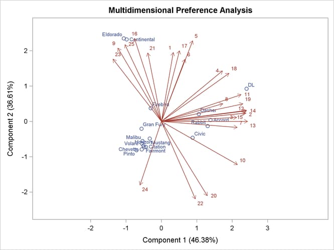
The biplot, shown in Output 92.1.3, is automatically displayed by PROC PRINQUAL when ODS Graphics is enabled and the MDPREF option is specified.
Output 92.1.3: Biplot Made with PRINQUAL
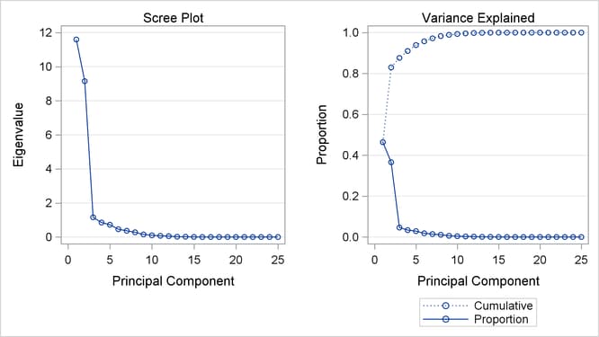
The second PROC PRINCOMP analysis is performed on the transformed data. The WHERE statement is used to retain only the monotonically transformed judgments. The scree plot shows that the first two eigenvalues are now much larger than the remaining smaller eigenvalues. The second eigenvalue has increased markedly at the expense of the next several eigenvalues. Two principal components seem to be necessary and sufficient to adequately describe these judges’ preferences for these automobiles. The cumulative proportion of variance displayed by PROC PRINCOMP for the first two principal components is 0.83. The following statements perform the analysis and produce Output 92.1.4:
* Final Principal Component Analysis;
proc princomp data=Results;
   ods select ScreePlot;
   var '1'n-'25'n;
   where _TYPE_='SCORE';
run;
Output 92.1.4: Transformed Data Eigenvalue Plot
The remainder of the example discusses the MDPREF biplot. A biplot is a plot that displays the relation between the row points
and the columns of a data matrix. The rows of , the standardized component scores, and , the structure matrix, contain enough information to reproduce . The  element of is the product of row i of and row j of . If all but the first two columns of and are discarded, the element of is approximated by the product of row i of and row j of .
Since the MDPREF analysis is based on a principal component model, the dimensions of the MDPREF biplot are the first two principal components. The first principal component is the longest dimension through the MDPREF biplot. The first principal component is overall preference, which is the most salient dimension in the preference judgments. One end points in the direction that is on the average preferred most by the judges, and the other end points in the least preferred direction. The second principal component is orthogonal to the first principal component, and it is the orthogonal direction that is the second most salient. The interpretation of the second dimension varies from example to example.
With an MDPREF biplot, it is geometrically appropriate to represent each automobile (object) by a point and each judge by a vector. The automobile points have coordinates that are the scores of the automobile on the first two principal components. The judge vectors emanate from the origin of the space and go through a point whose coordinates are the coefficients of the judge (variable) on the first two principal components.
The absolute length of a vector is arbitrary. However, the relative lengths of the vectors indicate fit, with the squared
lengths being proportional to the communalities that you can get in PROC FACTOR output. The direction of the vector indicates
the direction that is most preferred by the individual judge, with preference increasing as the vector moves from the origin.
Let  be row i of ,
  be row j of
  ,
,  be the length of
  ,
,  be the length of
  , and
, and  be the angle between and . The predicted degree of preference that an individual judge has for an automobile is
 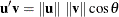 . Each automobile point can be orthogonally projected onto the vector. The projection of automobile i on vector j is
  , and the length of this projection is
  . The automobile that projects farthest along a vector in the direction it points is that judge’s most preferred automobile,
since the length of this projection, , differs from the predicted preference,
. The automobile that projects farthest along a vector in the direction it points is that judge’s most preferred automobile,
since the length of this projection, , differs from the predicted preference,  , only by , which is constant for each judge.
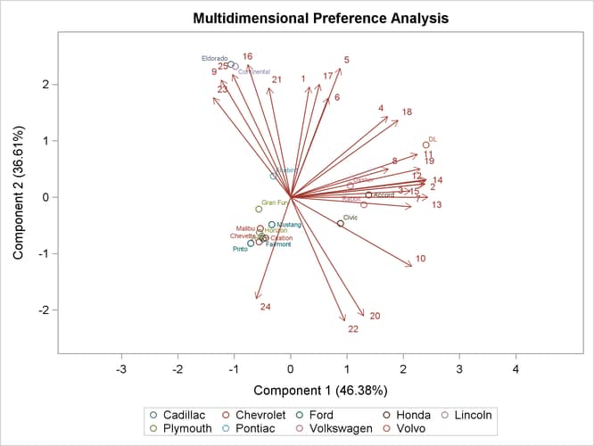
To interpret the biplot, look for directions through the plot that show a continuous change in some attribute of the automobiles, or look for regions in the plot that contain clusters of automobile points and determine what attributes the automobiles have in common. Points that are tightly clustered in a region of the plot represent automobiles that have the same preference patterns across the judges. Vectors that point in roughly the same direction represent judges who have similar preference patterns.
In the biplot, American automobiles are located at the left of the space, while European and Japanese automobiles are located at the right. At the top of the space are expensive American automobiles (Cadillac Eldorado, Lincoln Continental), while at the bottom are inexpensive ones (Ford Pinto, Chevrolet Chevette). The first principal component differentiates American from imported automobiles, and the second arranges automobiles by price and other associated characteristics.
The two expensive American automobiles form a cluster, the sporty automobile (Pontiac Firebird) is by itself, the Volvo DL is by itself, and the remaining imported autos form a cluster, as do the remaining American autos. It seems there are 5 prototypical automobiles in this set of 17, in terms of preference patterns among the 25 judges.
Most of the judges prefer the imported automobiles, especially the Volvo. There is also a fairly large minority that prefer the expensive autos, whether or not they are American (those with vectors that point toward one o’clock), or simply prefer expensive American automobiles (vectors that point toward eleven o’clock). There are two judges who prefer anything except expensive American autos (five o’clock vectors), and one who prefers inexpensive American autos (seven o’clock vector).
Several vectors point toward the upper-right corner of the plot, toward a region with no automobiles. This is the region between the European and Japanese autos at the right and the luxury autos at the top. This suggests that there is a market for luxury Japanese and European automobiles.
The next part of this example modifies the graph template for the MDPREF plot to display group information (the make of the automobile) in the MDPREF plot. First you need to run the PROC PRINQUAL step with ODS trace output enabled to find the name of the graph template for the MDPREF plot:
ods trace on;
proc prinqual data=CarPref out=Results n=2 replace mdpref;
   title2 'Multidimensional Preference (MDPREF) Analysis';
   title3 'Optimal Monotonic Transformation of Preference Data';
   id model;
   transform monotone('1'n-'25'n);
run;
The results are as follows:
Output Added:
-------------
Name:       MDPrefPlot
Label:      2 by 1
Template:   Stat.Prinqual.Graphics.MDPref
Path:       Prinqual.MDPREF.MDPrefPlot
-------------
The following step displays the template:
proc template;
   source Stat.Prinqual.Graphics.MDPref;
run;
The following template is displayed:
define statgraph Stat.Prinqual.Graphics.MDPref;
   notes "Multidimensional Preference Analysis Plot";
   dynamic xVar yVar xVec yVec ylab xlab yshortlab xshortlab xOri yOri
      stretch;
   begingraph;
      entrytitle "Multidimensional Preference Analysis";
      layout overlayequated / equatetype=fit xaxisopts=(label=XLAB shortlabel
         =XSHORTLAB offsetmin=0.1 offsetmax=0.1) yaxisopts=(label=YLAB
         shortlabel=YSHORTLAB offsetmin=0.1 offsetmax=0.1);
         scatterplot y=YVAR x=XVAR / datalabel=IDLAB1 rolename=(_tip1=
            OBSNUMVAR _id2=IDLAB2 _id3=IDLAB3 _id4=IDLAB4 _id5=IDLAB5 _id6=
            IDLAB6 _id7=IDLAB7 _id8=IDLAB8 _id9=IDLAB9 _id10=IDLAB10 _id11=
            IDLAB11 _id12=IDLAB12 _id13=IDLAB13 _id14=IDLAB14 _id15=IDLAB15
            _id16=IDLAB16 _id17=IDLAB17 _id18=IDLAB18 _id19=IDLAB19 _id20=
            IDLAB20) tip=(y x datalabel _tip1 _id2 _id3 _id4 _id5 _id6 _id7
            _id8 _id9 _id10 _id11 _id12 _id13 _id14 _id15 _id16 _id17 _id18
            _id19 _id20) datalabelattrs=GRAPHVALUETEXT (color=
            GraphData1:ContrastColor) markerattrs=GRAPHDATA1;
         vectorplot y=YVEC x=XVEC xorigin=0 yorigin=0 / datalabel=LABEL2VAR
            shaftprotected=false rolename=(_tip1=VNAME _tip2=VLABEL _tip3=
            YORI _tip4=XORI _tip5=LENGTH _tip6=LENGTH2) tip=(y x datalabel
            _tip1 _tip2 _tip3 _tip4 _tip5 _tip6) datalabelattrs=
            GRAPHVALUETEXT (color=GraphData2:ContrastColor) lineattrs=
            GRAPHDATA2 (pattern=solid) primary=true;
         if (0)
            entry "Vector Stretch = " STRETCH / autoalign=(topright topleft
               bottomright bottomleft right left top bottom);
         endif;
      endlayout;
   endgraph;
end;
The following step adds a PROC PRINQUAL statement and a RUN statement, removes attribute options from the SCATTERPLOT statement, adds a GROUP=IDLAB2 option to use the second ID variable as a group variable, and adds a NAME='s' option along with a DISCRETELEGEND statement to display the groups in a legend:
proc template;
   define statgraph Stat.Prinqual.Graphics.MDPref;
      notes "Multidimensional Preference Analysis Plot";
      dynamic xVar yVar xVec yVec ylab xlab yshortlab xshortlab xOri yOri
         stretch;
      begingraph;
         entrytitle "Multidimensional Preference Analysis";
         layout overlayequated / equatetype=fit xaxisopts=(label=XLAB shortlabel
            =XSHORTLAB offsetmin=0.1 offsetmax=0.1) yaxisopts=(label=YLAB
            shortlabel=YSHORTLAB offsetmin=0.1 offsetmax=0.1);
            scatterplot y=YVAR x=XVAR / datalabel=IDLAB1 rolename=(_tip1=
               OBSNUMVAR _id2=IDLAB2 _id3=IDLAB3 _id4=IDLAB4 _id5=IDLAB5 _id6=
               IDLAB6 _id7=IDLAB7 _id8=IDLAB8 _id9=IDLAB9 _id10=IDLAB10 _id11=
               IDLAB11 _id12=IDLAB12 _id13=IDLAB13 _id14=IDLAB14 _id15=IDLAB15
               _id16=IDLAB16 _id17=IDLAB17 _id18=IDLAB18 _id19=IDLAB19 _id20=
               IDLAB20) tip=(y x datalabel _tip1 _id2 _id3 _id4 _id5 _id6 _id7
               _id8 _id9 _id10 _id11 _id12 _id13 _id14 _id15 _id16 _id17 _id18
               _id19 _id20)

               group=idlab2 name='s'; *<==== add the group variable ====<<<<;

            vectorplot y=YVEC x=XVEC xorigin=0 yorigin=0 / datalabel=LABEL2VAR
               shaftprotected=false rolename=(_tip1=VNAME _tip2=VLABEL _tip3=
               YORI _tip4=XORI _tip5=LENGTH _tip6=LENGTH2) tip=(y x datalabel
               _tip1 _tip2 _tip3 _tip4 _tip5 _tip6) datalabelattrs=
               GRAPHVALUETEXT (color=GraphData2:ContrastColor) lineattrs=
               GRAPHDATA2 (pattern=solid) primary=true;

            discretelegend 's'; *<==== add a legend ====<<<<;

            if (0)
               entry "Vector Stretch = " STRETCH / autoalign=(topright topleft
                  bottomright bottomleft right left top bottom);
            endif;
         endlayout;
      endgraph;
   end;
run;
The following step creates the MDPREF plot with the make of the automobile added as a second ID variable and displayed in the graph as a group variable:
proc prinqual data=CarPref out=Results n=2 replace mdpref;
   title2 'Multidimensional Preference (MDPREF) Analysis';
   title3 'Optimal Monotonic Transformation of Preference Data';
   id model make;
   transform monotone('1'n-'25'n);
run;
The results are displayed in Output 92.1.5.
Output 92.1.5: Biplot with a Group Variable
The following step restores the default template:
proc template;
   delete Stat.Prinqual.Graphics.MDPref / store=sasuser.templat;
run;