The PLM Procedure

Example 87.3 Group Comparisons in an Ordinal Model

This example continues the study of the effects on taste of various cheese additives. You have finished fitting an ordinal logistic model and saved it to an item store named sasuser.cheese in the previous example. Suppose you want to make comparisons between any pair of cheese additives. You can conduct the analysis by using the ESTIMATE statement and constructing an appropriate $\mb{L}$ matrix, or by using the LSMEANS statement to compute least squares means differences. For an ordinal logistic model with the cumulative logit link, the least squares means are predicted population margins of the cumulative logits. The following statements compute and display differences between least squares means of cheese additive:

ods graphics on;
proc plm restore=sasuser.cheese;
   lsmeans additive / cl diff oddsratio plot=diff;
run;
ods graphics off;

The LSMEANS statement contains four options. The DIFF option requests least squares means differences for cheese additives. Since the fitted model is an ordinal logistic model with the cumulative logit link, the least squares means differences represent log cumulative odds ratios. The ODDSRATIO option requests exponentiation of the LS-means differences which produces cumulative odds ratios. The CL option constructs confidence limits for the LS-means differences. When ODS Graphics is enabled, the PLOTS=DIFF option requests a display of all pairwise least squares means differences and their significance.

Output 87.3.1 displays the LS-means differences. The reported log odds ratios indicate the relative difference among the cheese additives. A negative log odds ratio indicates that the first category (displayed in the Additive column) having a lower taste rating is less likely than the second category (displayed in the _Additive column) having a lower taste rating. For example, the log odds ratio between cheese additive 1 and 2 is –3.3517 and the corresponding odds ratio is 0.035. This means the odds of cheese additive 1 receiving a poor rating is 0.035 times the odds of cheese additive 2 receiving a poor rating. In addition to the highly significant p-value (< 0.0001), the confidence limits for both the log odds ratio and the odds ratio indicate that you can reject the null hypothesis that the odds of cheese additive 1 having a lower taste rating is the same as that of cheese additive 2 having a lower rating. Similarly, the odds of cheese additive 2 having a lower rating is 143.241 (with 95% confidence limits 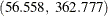$(56.558,~ 362.777)$ ) times the odds of cheese additive 4 having a lower rating. With the same logic, you can conclude that the preference order for the four cheese types from the most favorable to the least favorable is: 4, 1, 3 and 2.

Output 87.3.1: LS-Means Differences of Additive

Ordinal Model on Cheese Additives

The PLM Procedure

Differences of Additive Least Squares Means
Additive	_Additive	Estimate	Standard Error	z Value	Pr > \|z\|	Alpha	Lower	Upper	Odds Ratio	Lower Confidence Limit for Odds Ratio	Upper Confidence Limit for Odds Ratio
1	2	-3.3517	0.4235	-7.91	<.0001	0.05	-4.1818	-2.5216	0.035	0.015	0.080
1	3	-1.7098	0.3731	-4.58	<.0001	0.05	-2.4410	-0.9787	0.181	0.087	0.376
1	4	1.6128	0.3778	4.27	<.0001	0.05	0.8724	2.3532	5.017	2.393	10.520
2	3	1.6419	0.3738	4.39	<.0001	0.05	0.9092	2.3746	5.165	2.482	10.746
2	4	4.9645	0.4741	10.47	<.0001	0.05	4.0353	5.8938	143.241	56.558	362.777
3	4	3.3227	0.4251	7.82	<.0001	0.05	2.4895	4.1558	27.734	12.055	63.805

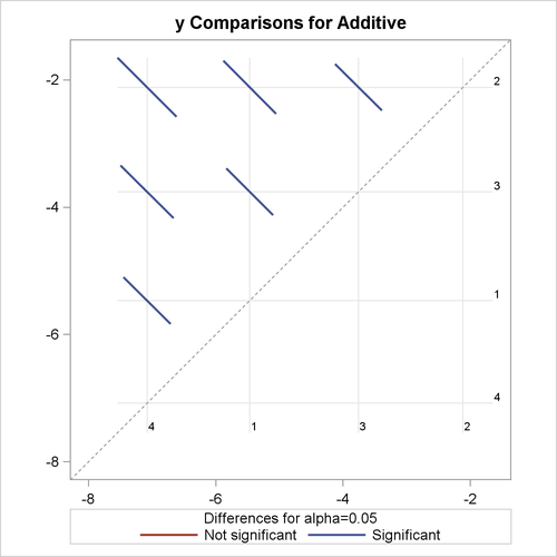
Output 87.3.2 displays the DiffPlot. This shows that all pairs of LS-means differences, equivalent to log odds ratios in this case, are significant at the level of $\alpha =0.05$ . This means that the preference between any pair of the four cheese additive types are statistically significantly different.

Output 87.3.2: LS-Means Plot of Pairwise Differences