The MULTTEST Procedure

Statistical Tests
The following section discusses the statistical tests performed in the MULTTEST procedure. For continuous data, a t test for the mean (MEAN ) is available. For discrete variables, available tests are the Cochran-Armitage linear trend test (CA ), the Freeman-Tukey double arcsine test (FT ), the Peto mortality-prevalence test (PETO ), and the Fisher exact test (FISHER ).
Throughout this section, the discrete and continuous variables are denoted by  and
and  , respectively, where v is the variable, g is the treatment group, s is the stratum, and r is the replication. Let
  denote the sample size for a binary variable v within group g and stratum s. A plus sign (+) subscript denotes summation over an index. Note that the tests are invariant to the location and scale of
the contrast coefficients
denote the sample size for a binary variable v within group g and stratum s. A plus sign (+) subscript denotes summation over an index. Note that the tests are invariant to the location and scale of
the contrast coefficients  .
.
Cochran-Armitage Linear Trend Test
The Cochran-Armitage linear trend test (Cochran 1954; Armitage 1955; Agresti 2002) is implemented by using a Z-score approximation , an exact permutation distribution , or a combination of both.
Z-Score Approximation
The pooled probability estimate for variable v and stratum s is
![\[ p_{vs} = \frac{S_{v+s+}}{m_{v+s}} \]](images/statug_multtest0072.png)
The expected value (under constant within-stratum treatment probabilities) for variable v, group g, and stratum s is
![\[ E_{vgs} = m_{vgs} p_{vs} \]](images/statug_multtest0073.png)
Letting denote the contrast trend coefficients specified by the CONTRAST
statement, the test statistic for variable v has numerator
![\[ N_ v = \sum _{s} \sum _{g} t_ g (S_{vgs+} - E_{vgs}) \]](images/statug_multtest0074.png)
The binomial variance estimate for this statistic is
![\[ V_ v = \sum _{s} p_{vs} (1 - p_{vs}) \sum _{g} m_{vgs} (t_ g - {\bar{t}}_{vs})^2 \]](images/statug_multtest0075.png)
where
![\[ {\bar{t}}_{vs} = \sum _{g} \frac{m_{vgs} t_ g}{m_{v+s}} \]](images/statug_multtest0076.png)
The hypergeometric variance estimate (the default) is
![\[ V_ v = \sum _{s} \{ m_{v+s}/(m_{v+s}-1)\} p_{vs} (1 - p_{vs}) \sum _{g} m_{vgs} (t_ g - {\bar{t}}_{vs})^2 \]](images/statug_multtest0077.png)
For any strata s with  , the contribution to the variance is taken to be zero.
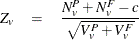
PROC MULTTEST computes the Z-score statistic
![\[ Z_ v = \frac{N_ v}{\sqrt {V_ v}} \]](images/statug_multtest0079.png)
The p-value for this statistic comes from the standard normal distribution. Whenever a 0 is computed for the denominator, the p-value is set to 1. This p-value approximates the probability obtained from the exact permutation distribution, discussed in the following text.
The Z-score statistic can be continuity-corrected to better approximate the permutation distribution. With continuity correction c, the upper-tailed p-value is computed from
![\[ Z_ v = \frac{N_ v - c}{\sqrt {V_ v}} \]](images/statug_multtest0080.png)
For two-tailed, noncontinuity-corrected tests, PROC MULTTEST reports the p-value as  , where p is the upper-tailed p-value. The same formula holds for the continuity-corrected test, with the exception that when the noncontinuity-corrected
Z and the continuity-corrected Z have opposite signs, the two-tailed p-value is 1.
, where p is the upper-tailed p-value. The same formula holds for the continuity-corrected test, with the exception that when the noncontinuity-corrected
Z and the continuity-corrected Z have opposite signs, the two-tailed p-value is 1.
When the PERMUTATION= option is specified and no STRATA variable is specified, PROC MULTTEST uses a continuity correction selected to optimally approximate the upper-tail probability of permutation distributions with smaller marginal totals (Westfall and Lin 1988). Otherwise, the continuity correction is specified by the CONTINUITY= option in the TEST statement.
The CA Z-score statistic is the Hoel-Walburg (Mantel-Haenszel) statistic reported by Dinse (1985).
Exact Permutation Test
When you use the PERMUTATION= option for CA in the TEST statement, PROC MULTTEST computes the exact permutation distribution of the trend score
![\[ T_ v = \sum _{s}\sum _{g} t_ g S_{vgs+} \]](images/statug_multtest0082.png)
where the contrast trend coefficients must be integer valued. The observed value of this trend is compared to the permutation distribution to obtain the p-value
![\[ p_ v = \Pr (X \ge \mbox{ observed } T_ v) \]](images/statug_multtest0083.png)
where X is a random variable from the permutation distribution and where upper-tailed tests are requested. This probability can be
viewed as a binomial probability, where the within-stratum probabilities are constant and where the probability is conditional
with respect to the marginal totals  . It also can be considered a rerandomization probability.
Because the computations can be quite time-consuming with large data sets, specifying the PERMUTATION= number option in the TEST statement limits the situations where PROC MULTTEST computes the exact permutation distribution. When marginal total success or total failure frequencies exceed number for a particular stratum, the permutation distribution is approximated by a continuity-corrected normal distribution. You should be cautious when using the PERMUTATION= option in conjunction with bootstrap resampling because the permutation distribution is recomputed for each bootstrap sample. This recomputation is not necessary with permutation resampling.
The permutation distribution is computed in two steps:
-
The permutation distributions of the trend scores are computed within each stratum.
-
The distributions are convolved to obtain the distribution of the total trend.
As long as the total success or failure frequency does not exceed number for any stratum, the computed distributions are exact. In other words, if  number or
  number for all s, then the permutation trend distribution for variable v is computed exactly.
In step 1, the distribution of the within-stratum trend
![\[ \sum _{g} t_ g S_{vgs+} \]](images/statug_multtest0087.png)
is computed by using the multivariate hypergeometric distribution of the  , provided number is not exceeded. This distribution can be written as
![\[ \Pr (S_{v1s+}, S_{v2s+},\ldots , S_{vGs+}) = \prod ^{G}_{g=1} \frac{ \left( \begin{array}{cc} m_{vgs} \\ S_{vgs+} \end{array} \right) }{ \left( \begin{array}{cc} m_{v+s} \\ S_{v+s+} \end{array} \right) } \]](images/statug_multtest0089.png)
The distribution of the within-stratum trend is then computed by summing these probabilities over appropriate configurations. For further information about this technique, see Bickis and Krewski (1986) and Westfall and Lin (1988). In step 2, the exact convolution distribution is obtained for the trend statistic summed over all strata having totals that meet the threshold criterion. This distribution is obtained by applying the fast Fourier transform to the exact within-stratum distributions. A description of this general method can be found in Pagano and Tritchler (1983) and Good (1987).
The convolution distribution of the overall trend is then computed by convolving the exact distribution with the distribution
of the continuity-corrected standard normal approximation. To be more specific, let  denote the subset of stratum indices that satisfy the threshold criterion, and let
  denote the subset of indices that do not satisfy the criterion. Let
  denote the combined trend statistic from the set , which has an exact distribution obtained from Fourier analysis as previously outlined, and let denote the combined trend statistic from the set . Then the distribution of the overall trend
  is obtained by convolving the analytic distribution of with the continuity-corrected normal approximation for
  . Using the notation from the section Z-Score Approximation, this convolution can be written as
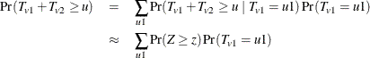
where Z is a standard normal random variable, and
![\[ z = \frac{1}{\sqrt {V_ v}} \left(u - u1 - \sum _{S_2} p_{vs} \sum _{g} t_ g m_{vgs} - c \right) \]](images/statug_multtest0096.png)
In this expression, the summation of s in  is over , and c is the continuity correction discussed under the Z-score approximation.
When a two-tailed test is requested, the expected trend is computed
![\[ E_ v = \sum _{s} \sum _{g} t_ g E_{vgs} \]](images/statug_multtest0098.png)
The two-tailed p-value is reported as the permutation tail probability for the observed trend  plus the permutation tail probability for
  , the reflected trend.
Freeman-Tukey Double Arcsine Test
For this test, the contrast trend coefficients  are centered to the values
  , where
  ,
,  , and G is the number of groups. The numerator of this test statistic is
![\[ N_ v = \sum _{s} w_{vs} \sum _{g} c_{g} f(S_{vgs+} , m_{vgs}) \]](images/statug_multtest0105.png)
where the weights  take on three different types of values depending upon your specification of the WEIGHT=
option in the STRATA
statement. The default value is the within-strata sample size
take on three different types of values depending upon your specification of the WEIGHT=
option in the STRATA
statement. The default value is the within-strata sample size  , ensuring comparability with the ordinary CA trend statistic. WEIGHT=
HARMONIC sets equal to the harmonic mean
, ensuring comparability with the ordinary CA trend statistic. WEIGHT=
HARMONIC sets equal to the harmonic mean
![\[ \left[ \left( \sum _{g} \frac{1}{m_{vgs}} \right) / G^* \right]^{-1} \]](images/statug_multtest0108.png)
where  is the number of nonmissing groups and the summation is over only the nonmissing elements. The harmonic means analysis places
more weight on the smaller sample sizes than does the default sample size method, and is similar to a Type 2 analysis in PROC
GLM. WEIGHT=
EQUAL sets
is the number of nonmissing groups and the summation is over only the nonmissing elements. The harmonic means analysis places
more weight on the smaller sample sizes than does the default sample size method, and is similar to a Type 2 analysis in PROC
GLM. WEIGHT=
EQUAL sets  for all v and s, and is similar to a Type 3 analysis in PROC GLM.
The function  is the double arcsine transformation:
![\[ f(r,n) = \arcsin \left( \sqrt { \frac{r}{n+1} } \right) + \arcsin \left( \sqrt { \frac{r+1}{n+1} } \right) \]](images/statug_multtest0112.png)
The variance estimate is
![\[ V_ v = \sum _{s} w_{vs}^2 \sum _{g} \frac{c_ g^2}{m_{vgs} + \frac{1}{2}} \]](images/statug_multtest0113.png)
The test statistic is
The Freeman-Tukey transformation and its variance are described by Freeman and Tukey (1950) and Miller (1978). Since its variance is not weighted by the pooled probabilities, as is the CA test, the FT test can be more useful than the CA test for tests involving only a subset of the groups.
Peto Mortality-Prevalence Trend Test
The Peto test is a modified Cochran-Armitage procedure incorporating mortality and prevalence information. The Peto test is computed like two Cochran-Armitage Z-score approximations, one for prevalence and one for mortality (Peto et al. 1980). It represents a special case in PROC MULTTEST because the data structure requirements are different, and the resampling methods used for adjusting p-values are not valid. The TIME= option variable is required to specify "death" times or, more generally, times of occurrence. In addition, the test variables must assume one of the following three values:
-
0 = no occurrence
-
1 = incidental occurrence
-
2 = fatal occurrence
Use the TIME= option variable to define the mortality strata, and use the STRATA statement variable to define the prevalence strata.
In the following notation, the subscript v represents the variable, g represents the treatment group, s represents the stratum, and t represents the time. Recall that a plus sign  in a subscript location denotes summation over that subscript.
Let  be the number of incidental occurrences, and let
  be the total sample size for variable v in group g, stratum s, excluding fatal tumors.
Let  be the number of fatal occurrences in time period t, and let
  be the number of patients alive at the end of time t – 1.
The pooled probability estimates are given by

The expected values are
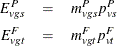
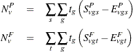
Let denote a contrast trend coefficient, and define the numerator terms as follows:
Define the denominator variance terms by using the binomial variance:
![\begin{eqnarray*} V_ v^ P & = & \sum _{s} p^ P_{vs} \left(1 - p^ P_{vs}\right) \left[ \left( \sum _{g} m^ P_{vgs} {t_ g}^2 \right) - \frac{1}{m^ P_{v+s}} \left( \sum _{g} m^ P_{vgs} t_ g \right)^2 \right] \\ V_ v^ F & = & \sum _{s} p^ F_{vt} \left(1 - p^ F_{vt}\right) \left[ \left( \sum _{g} m^ F_{vgt} {t_ g}^2 \right) - \frac{1}{m^ F_{v+t}} \left( \sum _{g} m^ F_{vgt} t_ g \right)^2 \right] \\ \end{eqnarray*}](images/statug_multtest0122.png)
The hypergeometric variances (the default) are calculated by weighting the within-strata variances as discussed in the section Z-Score Approximation.
The Peto statistic is computed as
where c is a continuity correction. The p-value is determined from the standard normal distribution unless the PERMUTATION=
number option is used. When you use the PERMUTATION=
option for PETO
in the TEST
statement, PROC MULTTEST computes the "discrete approximation" permutation distribution described by Mantel (1980) and Soper and Tonkonoh (1993). Specifically, the permutation distribution of 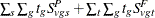 is computed, assuming that
  and
and  are independent over all s and t. Note that the contrast trend coefficients must be integer valued. The p-values are exact under this independence assumption. However, the independence assumption is valid only asymptotically, which
is why these p-values are called "approximate."
are independent over all s and t. Note that the contrast trend coefficients must be integer valued. The p-values are exact under this independence assumption. However, the independence assumption is valid only asymptotically, which
is why these p-values are called "approximate."
An exact permutation distribution is available only under the assumption of equal risk of censoring in all treatment groups; even then, computing this distribution can be cumbersome. Soper and Tonkonoh (1993) describe situations where the discrete approximation distribution closely fits the exact permutation distribution.
Fisher Exact Test
The CONTRAST statement in PROC MULTTEST enables you to compute Fisher exact tests for two-group comparisons. No stratification variable is allowed for this test. Note, however, that the FISHER exact test is a special case of the exact permutation tests performed by PROC MULTTEST and that these permutation tests allow a stratification variable. Recall that contrast coefficients can be –1, 0, or 1 for the Fisher test. The frequencies and sample sizes of the groups scored as –1 are combined, as are the frequencies and sample sizes of the groups scored as 1. Groups scored as 0 are excluded. The –1 group is then compared with the 1 group by using the Fisher exact test.
Letting x and m denote the frequency and sample size of the 1 group, and letting y and n denote those of the –1 group, the p-value is calculated as
![\[ \Pr (X \ge x ~ |~ X + Y = x + y) = \sum ^{m}_{i=x} \frac{ \left( \begin{array}{cc} m \\ i \end{array} \right) \left( \begin{array}{cc} n \\ x + y - i \end{array} \right) }{ \left( \begin{array}{cc} m + n \\ x + y \end{array} \right) } \]](images/statug_multtest0127.png)
where X and Y are independent binomially distributed random variables with sample sizes m and n and common probability parameters. The hypergeometric distribution is used to determine the stated probability; Yates (1984) discusses this technique. PROC MULTTEST computes the two-tailed p-values by adding probabilities from both tails of the hypergeometric distribution. The first tail is from the observed x and y, and the other tail is chosen so that the resulting probability is as large as possible without exceeding the probability from the first tail. If the variable being tested has only one level, then the p-value is set to 1.
t Test for the Mean
For continuous variables, PROC MULTTEST automatically centers the contrast trend coefficients, as in the Freeman-Tukey test.
These centered coefficients  are then used to form a t statistic contrasting the within-group means. Let
  denote the sample size within group g and stratum s; it depends on variable v only when there are missing values. Determine the weights as in the Freeman-Tukey test with replacing . Define
![\[ {\bar{X}}_{vgs+} = \frac{1}{n_{vgs}} \sum _{r}X_{vgsr} \]](images/statug_multtest0130.png)
as the sample mean within a group-and-stratum combination, and let  denote the treatment means. Write the null hypothesis as
![\[ \sum _{s} w_{vs} \sum _{g} c_ g \mu _{vgs} = 0 \]](images/statug_multtest0132.png)
Also define
![\[ s_ v^2 = \frac{\displaystyle \sum _{s}\sum _{g}\sum _{r} \left(X_{vgsr}-{\bar{X}}_{vgs+} \right)^2 }{\displaystyle \sum _{s}\sum _{g}\left( n_{vgs} - 1 \right)} \]](images/statug_multtest0133.png)
as the pooled sample variance.
Homogeneous Variance
Assuming constant variance for all group-and-stratum combinations, the t statistic for the mean is
![\[ M_ v = \frac{\displaystyle \sum _{s} w_{vs} \sum _{g}c_ g {\bar{X}}_{vgs+}}{\displaystyle \sqrt { s_ v^2 \left(\sum _{s} w_{vs}^2 \sum _{g}\frac{c_ g^2}{n_{vgs}} \right) } } \]](images/statug_multtest0134.png)
Then under the null hypothesis and assuming normality, independence, and homoscedasticity,  follows a t distribution with
 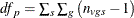 degrees of freedom.
Whenever a denominator of 0 is computed, the p-value is set to 1. When missing data force  , the contribution to the denominator of the pooled variance is 0 and not –1. This is also true for the degrees of freedom.
Heterogeneous Variance
If you do not assume constant variance for all group-and-stratum combinations, then the approximate t test is
![\[ M_ v = \frac{\displaystyle \sum _{s}w_{vs}\sum _{g} c_ g \bar{X}_{vgs+}}{\displaystyle \sqrt {\sum _{s}w_{vs}^2\sum _{g} c_ g^2 \frac{\displaystyle s_{vgs}^2}{\displaystyle n_{vgs}} }} \]](images/statug_multtest0138.png)
Under the null hypothesis and assuming normality and independence, the Satterthwaite (1946) approximation for the degrees of freedom of the t test is given by
![\[ \mathit{df}_ s = \frac{\displaystyle \left( \sum _{s}w_{vs}^2\sum _{g} c_ g^2 \frac{\displaystyle s_{vgs}^2}{\displaystyle n_{vgs}} \right)^2 }{\displaystyle \sum _{s} \sum _{g} \frac{\displaystyle \left( w_{vs}^2c_ g^2 \frac{\displaystyle s_{vgs}^2}{\displaystyle n_{vgs}} \right)^2}{\displaystyle n_{vgs}-1}} \]](images/statug_multtest0139.png)
under the restriction 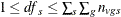 .
.
Whenever a denominator of 0 for is computed, the p-value is set to 1. If the denominator for  is computed as 0, then set
  . When missing data force
  , that group-and-stratum combination does not contribute to the computation.