The MIANALYZE Procedure

This example illustrates sensitivity analysis in multiple imputation under the MNAR assumption in which you search for a tipping point that reverses the study conclusion.

Suppose that a pharmaceutical company is conducting a clinical trial to test the efficacy of a new drug. The trial is conducted with two groups that have an equal number of patients: a treatment group that receives the new drug and a placebo control group. The variable Trt is an indicator variable, with a value of 1 for patients in the treatment group and a value of 0 for patients in the control group. The variable Y0 is the baseline efficacy score, and the variable Y1 is the efficacy score at a follow-up visit.

If the data set does not contain any missing values, then you can use a regression model such as the following to test the efficacy of the treatment effect:

Now suppose in a trial that the variables Trt and Y0 are fully observed and the variable Y1 contains missing values in both the treatment and control groups. The data set Mono2 contains the data from the trial and Output 76.13.1 lists the first 10 observations.

Multiple imputation often assumes that missing values are missing at random (MAR), and the following statements use the MI procedure to impute missing values under this assumption:

proc mi data=Mono2 seed=14823 out=outmi;
   class Trt;
   monotone reg;
   var Trt y0 y1;
run;

The following statements generate regression coefficients for each of the 25 imputed data sets:

ods select none;
proc reg data=outmi;
   model y1= Trt y0;
   by  _Imputation_;
   ods output parameterestimates=regparms;
run;
ods select all;

Because of the ODS SELECT statements, no output is displayed. The following statements combine the 20 sets of regression coefficients:

proc mianalyze parms=regparms;
   modeleffects Trt;
run;

The "Parameter Estimates" table in Output 76.13.2 displays a combined estimate and standard error for the regression coefficient for Trt. The table displays a 95% confidence interval (0.3353, 1.3208), which does not contain 0. The table also shows a t statistic of 3.31, with the associated p-value 0.0011 for the test that the regression coefficient is equal to 0.

The conclusion in Output 76.13.2 is based on the MAR assumption. But if it is plausible that, for the treatment group, the distribution of missing Y1 responses has a lower expected value than that of the corresponding distribution of the observed Y1 responses, the conclusion under the MAR assumption should be examined.

The following macro performs multiple imputation analysis for a specified sequence of shift parameters, which adjust the imputed values for observations in the treatment group (TRT=1):

/*---------------------------------------------------------*/
/*--- Performs multiple imputation analysis             ---*/
/*--- for specified shift parameters:                   ---*/
/*--- data= input data set                              ---*/
/*--- smin= min shift parameter                         ---*/
/*--- smax= max shift parameter                         ---*/
/*--- sinc= increment of the shift parameter            ---*/
/*--- outparms= output reg parameters                   ---*/
/*---------------------------------------------------------*/
%macro miparms( data=, smin=, smax=, sinc=, outparms=);
ods select none;

data &outparms;
   set _null_;
run;

/*------------ # of shift values ------------*/
%let ncase= %sysevalf( (&smax-&smin)/&sinc, ceil );

/*---- Multiple imputation analysis for each shift ----*/
%do jc=0 %to &ncase;
   %let sj= %sysevalf( &smin + &jc * &sinc);

  /*---- Generates 25 imputed data sets ----*/
   proc mi data=&data seed=14823 out=outmi;
      class Trt;
      monotone reg;
      mnar adjust( y1 / shift=&sj  adjustobs=(Trt='1') );
      var Trt y0 y1;
   run;

  /*------ Perform reg test -------*/
   proc reg data=outmi;
      model y1= Trt y0;
      by  _Imputation_;
      ods output parameterestimates=regparm;
   run;

  /*------ Combine reg results -------*/
   proc mianalyze parms=regparm;
      modeleffects Trt;
      ods output parameterestimates=miparm;
   run;

   data miparm;
      set miparm;
      Shift= &sj;
      keep Shift Probt;
   run;

  /*----- Output multiple imputation results ----*/
   data &outparms;
      set &outparms miparm;
   run;

%end;

ods select all;
%mend miparms;

Assume that the tipping point for the shift parameter that reverses the study conclusion is between –3 and 0. The following statement performs multiple imputation analysis for each of the shift parameters –3.0, –2.9, …, 0:

%miparms( data=Mono2, smin=-3, smax=0, sinc=0.1, outparms=parm1);

The following statements display the plot of p-values for shift parameters between –3 and 0:

title 'P-value Plot';
proc sgplot data=parm1;
   series x=Shift y=Probt / lineattrs=graphfit(color=blue);
   refline 0.05 / axis=y lineattrs=graphfit(thickness=1px pattern=shortdash);
   xaxis label="Shift Parameter";
   yaxis label="P-value";
run;

Output 76.13.3: Finding Tipping Point for Shift Parameter between –3 and 0

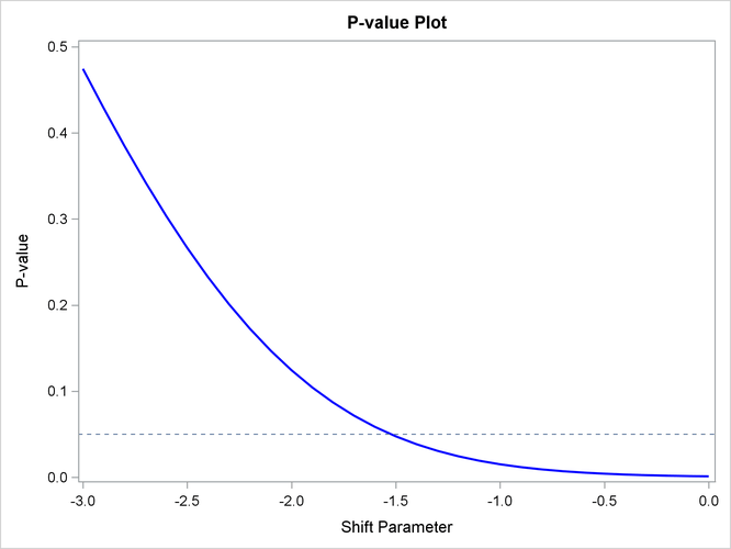
For a two-sided Type I error level of 0.05, the tipping point for the shift parameter is slightly less than –1.5. The following statement performs multiple imputation analysis for shift parameters –1.60, –1.59, …, –1.50:

%miparms( data=Mono2, smin=-1.6, smax=-1.5, sinc=0.01, outparms=parm2);

The following statements display the p-values that are associated with the shift parameters:

proc print label data=parm2;
   var Shift Probt;
   title 'P-values for Shift Parameters';
   label Probt='Pr > |t|';
   format Probt 8.4;
run;

The study conclusion under MAR is reversed when the shift parameter is –1.53. Thus, if the shift parameter –1.53 is plausible, the conclusion under MAR is questionable.