The LIFETEST Procedure

Analysis of Competing-Risks Data

Competing risks arise in studies in which individuals are exposed to two or more mutually exclusive failure events, denoted by $\delta \in \{ 1,\ldots ,J\}$ . When a failure occurs, you observe the time T and the cause of failure $\delta$ . The cumulative incidence function (CIF), also known as the subdistribution function, for failures of cause j is the probability

$F_ j(t)= \mr{Pr}(T\leq t, \delta =j)$

The nonparametric analysis of competing-risks data consists of estimating the CIF and comparing the CIFs of two or more groups.

Estimation of the CIF

For a set of competing-risks data with $J\geq 2$ causes of failure, let $t_1 < t_2 < \cdots < t_ L$ be the distinct uncensored times. For each $l=1, \ldots , L$ , let $Y_ l$ be the number of subjects at risk at $t_ l$ , and let $d_{jl}$ be the number of failures of cause j at $t_ l$ . Let $\hat{S}(t)$ be the Kaplan-Meier estimator that would have been obtained by assuming that all failure causes are of the same type. Denote $t_0=0$ .

The nonparametric maximum likelihood estimator of the CIF of cause j is

$\hat{F}_ j(t) = \sum _{t_ l \leq t} \frac{d_{ji}}{Y_ l} \hat{S}(t_{l-1})$

PROC LIFETEST provides two standard error estimators of the CIF estimator: one is based on the theory of counting processes (Aalen 1978), and the other is based on the delta method (Marubini and Valsecchi 1995). You use the ERROR= option in the PROC LIFETEST statement to choose the standard error estimator. The default is the Aalen estimator (ERROR=AALEN). Denote $d_{.l}=\sum _{j=1}^ J d_{jl}$ .

Aalen Estimator

$\begin{align*} \hat{\sigma }^2_{A}(\hat{F}_ j(t)) & = \sum _{t_ l\leq t} \left[\hat{F}_ j(t) - \hat{F}_ j(t_ l)\right]^2 \frac{d_{.l}}{(Y_ l-1)(Y_ l-d_{.l})} \\ & + \sum _{t_ l\leq t}\hat{S}^2(t_{l-1}) \frac{d_{kj}(Y_ l-d_{jl})}{Y_ l^2(Y_ l-1)} \\ & - 2 \sum _{t_ l\leq t}\left[\hat{F}_ j(t) - \hat{F}_ j(t_ l)\right] \hat{S}(t_{l-1}) \frac{d_{jl}(Y_ l-d_{jl})}{Y_ l(Y_ l-d_{.l})(Y_ l-1)} \end{align*}$

Delta Estimator

$\begin{align*} \hat{\sigma }^2_{D}(\hat{F}_ j(t)) & = \sum _{t_ l\leq t} \left[\hat{F}_ j(t) - \hat{F}_ j(t_ l)\right]^2 \frac{d_{.l} }{Y_ l(Y_ l-d_{.l})} \\ & + \sum _{t_ l\leq t}\hat{S}^2(t_{l-1}) \frac{d_{jl}(Y_ l-d_{jl})}{Y_ l^3} \\ & - 2 \sum _{t_ l\leq t} \left[\hat{F}_ j(t) - \hat{F}_ j(t_ l)\right] \hat{S}(t_{l-1})\frac{d_{jl}}{Y_ l^2} \end{align*}$

Comparison of the CIF of a Competing Risk for Two or More Groups

Let K be the number of groups. Consider failure of type 1 to be the failure type of interest. Let $F_{1k}$ be the cumulative incidence function of type 1 in group k. The null hypothesis to be tested is

$H_0: F_{11} = F_{12} = \cdots = F_{1K} \equiv F_1^0$

Gray (1988, Section 2) gives the following K-sample test procedure for testing $H_0$ . Let $(T_{ik},\delta _{ik}), i=1,\ldots ,n_ k$ be the observed data in the kth group. Without loss of generality, assume that there are only two types of failure ( $J=2$ ). The number of failures of type j by t is

$N_{jk}(t) = \sum _{i=1}^{n_ k} I(T_{ik} \leq t, \delta _{ik}=j), \mbox{~ ~ ~ }j=1,2$

and the number of subjects at risk just before t in group k is

$Y_ k(t) = \sum _{i=1}^{n_ k} I(T_{ik}\geq t)$

For group k, let $\hat{S}_ k(t)$ be the Kaplan-Meier estimator of the survivor function that you obtain by assuming that all failure causes are of the same type. The cumulative incidence function $F_{jk}(t)$ of type j in the kth group is estimated by

$\hat{F}_{jk}(t) = \int _0^ t \hat{S}_ k(u-)Y_ k^{-1}(u)dN_{jk}(u)$

Let $\tau _ k$ be the largest uncensored time in group k. Define

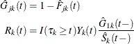
$\begin{align*} \hat{G}_{jk}(t) & = 1 - \hat{F}_{jk}(t) \\ R_ k(t) & = I(\tau _ k \geq t) Y_ k(t)\frac{\hat{G}_{1k}(t-)}{\hat{S}_ k(t-)} \end{align*}$

The cumulative hazard of the subdistribution for group k, $\Gamma _{1k}$ , is estimated by

$\hat{\Gamma }_{1k}(t)=\int _0^ t\frac{d\hat{F}_{1k}(u)}{\hat{G}_{1k}(u-)} =\int _0^ t\frac{dN_{1k}(u)}{R_{k}(u-)}, \mbox{~ ~ ~ }t\leq \tau _ k$

Under the null hypothesis $H_0$ , you can estimate the null value of $\Gamma _{1k}(t)$ , denoted by $\Gamma _1^0(t)$ , by

$\hat{\Gamma }^0_1(t)= \int _0^ t \frac{dN_{1.}(u)}{R_.(u)}$

The K-sample test is based on $\mb{z}=(z_1,\ldots ,z_{K})’$ , where

$z_ k = \int _0^{\tau _ k} R_ k(t)\left[d\hat{\Gamma }_{1k}(t)-d\hat{\Gamma }_1^0(t) \right]$

You can estimate the asymptotic covariance matrix $\Sigma =(\sigma _{kk'})$ as

$\hat{\sigma }^2_{kk'} = \sum _{r=1}^ K \int _0^{\tau _ k \wedge \tau _{k'}} \frac{a_{kr}(t) a_{k'r}(t)}{ \hat{h}_ r(t)} d\hat{F}_1^0(t) + \sum _{r=1}^ K \int _0^{\tau _ k \wedge \tau _{k'}} \frac{b_{2kr}(t) b_{2k'r}(t)}{ \hat{h}_ r(t)} d\hat{F}_{2r}(t)$

where

$\begin{eqnarray*} \hat{h}_ r(t) & =& \frac{I(t\leq \tau _ r)Y_ r(t)}{\hat{S}_ r(t-)} \\ \hat{F}_1^0(t) & =& \int _0^ t \frac{dN_{1.}(u)}{\hat{h}_{.}(u)}\\ \hat{G}_1^0(t) & =& 1 - \hat{F}_1^0(t)\\ a_{kr}(t) & =& d_{1kr}(t) + b_{1kr}(t) \\ b_{jkr}(t) & =& \left[ I(j=1) - \frac{\hat{G}^0_1(t)}{\hat{S}_ r(t)} \right] \left[ c_{kr}(\tau _ k) - c_{kr}(t) \right] \\ c_{kr}(t) & =& \int _0^ t d_{1kr}(u)d\hat{\Gamma }^0_1(u) \\ d_{jkr}(t) & =& I(j=1)R_ k(t) \frac{I(k=r) - \frac{\hat{h}_ r(t)}{\hat{h}_{.}(t)}}{\hat{G}^0_1(t)} \end{eqnarray*}$

Because $\sum _{k=1}^ Kz_ k=0$ , only $K-1$ scores are linearly independent. The K-sample test statistic is formed as a quadratic form of the first $K-1$ components of $\mb{z}$ and the inverse of the estimated covariance matrix. Under the null hypothesis $H_0$ , this K-sample test statistic has approximately a chi-square distribution with $K-1$ degrees of freedom.

If you specify the GROUP= option in the STRATA statement, you can obtain a stratified version of the test by computing the contributions to $z_ k$ and $\sigma ^2_{kk'}$ for each stratum, summing the contributions over the strata, and proceeding as before.