The LIFETEST Procedure

Comparison of Two or More Groups of Survival Data
Let K be the number of groups. Let  be the underlying survivor function of the kth group,
  . The null and alternative hypotheses to be tested are
 for all
versus
 at least one of the ’s is different for some
respectively, where  is the largest observed time.
Likelihood Ratio Test
The likelihood ratio test statistic (Lawless 1982) for test  versus
  assumes that the data in the various samples are exponentially distributed and tests that the scale parameters are equal.
The test statistic is computed as
assumes that the data in the various samples are exponentially distributed and tests that the scale parameters are equal.
The test statistic is computed as
![\[ \chi ^2 = 2N \log \left( \frac{T}{N} \right) - 2 \sum _{k=1}^ K N_ k \log \left( \frac{T_ k}{N_ k} \right) \]](images/statug_lifetest0205.png)
where  is the total number of events in the kth group,
  ,
,  is the total time on test in the kth stratum, and
  . The approximate probability value is computed by treating
  as having a chi-square distribution with K – 1 degrees of freedom.
Nonparametric Tests
Let (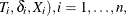 denote an independent sample of right-censored survival data, where
  is the possibly right-censored time,
  is the censoring indicator (=0 if is censored and =1 if is an event time), and
  for K different groups. Let
  be the distinct event times in the sample. At time
  let
let  be a positive weight function, and let
 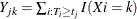 and
and 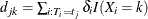 be the size of the risk set and the number of events in the kth group, respectively. Let
  ,
,  .
.
The choices of the weight function are given in Table 70.3.
Table 70.3: Weight Functions for Various Tests
|
Test |
|
|---|---|
|
Log-rank |
1.0 |
|
Wilcoxon |
|
|
Tarone-Ware |
|
|
Peto-Peto |
|
|
Modified Peto-Peto |
|
|
Harrington-Fleming (p,q) |
|


![$[\hat{S}(t_{j-1})]^ p[1-\hat{S}(t_{j-1})]^ q, p\ge 0, q\ge 0$](images/statug_lifetest0225.png)
In Table 70.3,  is the product-limit estimate at t for the pooled sample, and
  is a survivor function estimate close to given by
![\[ \tilde{S}(t) = \prod _{t_ j\le t} \biggl (1 - \frac{d_ j}{Y_ j+1} \biggr ) \]](images/statug_lifetest0227.png)
Unstratified Tests
The rank statistics (Klein and Moeschberger 1997, Section 7.3) for testing versus have the form of a K-vector 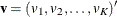 with
with
![\[ v_ k = \sum _{j=1}^ D \left[W(t_ j) \left( d_{jk} - Y_{jk}\frac{d_ j}{Y_ j} \right) \right] \]](images/statug_lifetest0229.png)
and the variance of  and the covariance of and
  are, respectively,
![\begin{eqnarray*} V_{kk} & =& \sum _{j=1}^ D \left[W^2(t_ j) \frac{ d_ j (Y_ j-d_ j) Y_{jk} (Y_ j - Y_{jk})}{ Y_ j^2 (Y_ j - 1) } \right], \mbox{~ ~ ~ } 1\leq k \leq K \\ V_{kh} & =& -\sum _{j=1}^ D \left[W^2(t_ j) \frac{ d_ j (Y_ j-d_ j) Y_{jk} Y_{jh} }{ Y_ j^2 (Y_ j - 1) }\right], \mbox{~ ~ ~ } 1 \leq k \neq h \leq K \end{eqnarray*}](images/statug_lifetest0232.png)
The statistic can be interpreted as a weighted sum of observed minus expected numbers of failure for the kth group under the null hypothesis of identical survival curves. Let  . The overall test statistic for homogeneity is
  , where
  denotes a generalized inverse of
  . This statistic is treated as having a chi-square distribution with degrees of freedom equal to the rank of for the purposes of computing an approximate probability level.
Adjusted Log-Rank Test
PROC LIFETEST computes the weighted log-rank test (Xie and Liu 2005, 2011) if you specify the WEIGHT statement. Let (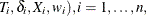 denote an independent sample of right-censored survival data, where is the possibly right-censored time, is the censoring indicator (=0 if is censored and =1 if is an event time), for K different groups, and
  is the weight from the WEIGHT statement. Let be the distinct event times in the sample. At each
  , and for each
  , let
, let
Let  and
and  denote the number of events and the number at risk, respectively, in the combined sample at time
  . Similarly, let
  and
and  denote the weighted number of events and the weighted number at risk, respectively, in the combined sample at time . The test statistic is
![\[ v_ k= \sum _{j=1}^ D \left( d^ w_{jk} - Y^ w_{jk} \frac{d^ w_ j}{Y^ w_ j} \right) \mbox{~ ~ }k= 1, \ldots , K \]](images/statug_lifetest0244.png)
and the variance of and the covariance of and are, respectively,
![\begin{eqnarray*} {V}_{kk} & = & \sum _{j=1}^ D \left\{ \frac{d_ j(Y_ j-d_ j)}{Y_ j(Y_ j-1)} \sum _{i=1}^{Y_ j} \left[ \left( \frac{Y^ w_{jk}}{Y^ w_ j }\right)^2 w^2_ iI\{ X_ i\neq k\} + \left( \frac{Y^ w_ j - Y^ w_{jk}}{Y^ w_ j }\right)^2 w^2_ i I\{ X_ i=k\} \right] \right\} , \mbox{~ ~ ~ } 1\leq k \leq K \\ {V}_{kh} & = & \sum _{j=1}^ D \left\{ \frac{d_ j(Y_ j-d_ j)}{Y_ j(Y_ j-1)} \sum _{i=1}^{Y_ j} \left[ \frac{Y^ w_{jk} Y^ w_{jh}}{(Y^ w_ j)^2} w^2_ iI\{ X_ i\neq k, h\} - \frac{(Y^ w_ j - Y^ w_{jk})Y^ w_{jh}}{(Y^ w_ j)^2} w^2_ i I\{ X_ i=k\} \right. \right. \\ & & \left. \left. - \frac{(Y^ w_ j - Y^ w_{jh})Y^ w_{jk}}{(Y^ w_ j)^2} w^2_ i I\{ X_ i=h\} \right] \right\} , \mbox{~ ~ ~ } 1 \leq k \neq h \leq K \end{eqnarray*}](images/statug_lifetest0245.png)
Let  . Under , the weighted K-sample test has a statistic given by
![\[ \chi ^2= (v_1,\ldots ,v_ K) \bV ^{-} (v_1,\ldots ,v_ K)’ \]](images/statug_lifetest0247.png)
with K – 1 degrees of freedom.
Stratified Tests
Suppose the test is to be stratified on M levels of a set of STRATA variables. Based only on the data of the sth stratum ( ), let
  be the test statistic (Klein and Moeschberger 1997, Section 7.5) for the sth stratum, and let
  be its covariance matrix. Let

A global test statistic is constructed as
![\[ \chi ^2 = \mb{v}’ \bV ^{-} \mb{v} \]](images/statug_lifetest0252.png)
Under the null hypothesis, the test statistic has a distribution with the same degrees of freedom as the individual test for each stratum.
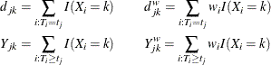
Multiple-Comparison Adjustments
Let  denote a chi-square random variable with r degrees of freedom. Denote
  and
and  as the density function and the cumulative distribution function of a standard normal distribution, respectively. Let m be the number of comparisons; that is,
For a two-sided test that compares the survival of the jth group with that of lth group,  , the test statistic is
![\[ z^2_{jl}= \frac{(v_ j - v_ l)^2}{V_{jj} + V_{ll} - 2V_{jl}} \]](images/statug_lifetest0257.png)
and the raw p-value is
![\[ p = \mr{Pr}(\chi ^2_1 > z^2_{jl}) \]](images/statug_lifetest0258.png)
Adjusted p-values for various multiple-comparison adjustments are computed as follows:
-
Bonferroni adjustment:
![\[ p = \mr{min}\{ 1, m \mr{Pr}(\chi ^2_1 > z^2_{jl})\} \]](images/statug_lifetest0259.png)
-
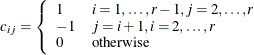
Dunnett-Hsu adjustment: With the first group being the control, let
 be the
  matrix of contrasts; that is,
Let
 and
and  be covariance and correlation matrices of
  , respectively; that is,
![\[ \bSigma = \bC \bV \bC ’ \]](images/statug_lifetest0266.png)
and
![\[ r_{ij}= \frac{\sigma _{ij}}{\sqrt {\sigma _{ii}\sigma _{jj}}} \]](images/statug_lifetest0267.png)
The factor-analytic covariance approximation of Hsu (1992) is to find
 such that
![\[ \bR = \bD + \blambda \blambda ’ \]](images/statug_lifetest0269.png)
where
 is a diagonal matrix with the jth diagonal element being
  and
and 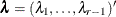 . The adjusted p-value is
![\[ p= 1 - \int _{-\infty }^{\infty } \phi (y) \prod _{i=1}^{r-1} \biggl [ \Phi \biggl (\frac{\lambda _ i y + z_{jl}}{\sqrt {1-\lambda _ i^2}}\biggr ) - \Phi \biggl (\frac{\lambda _ i y - z_{jl}}{\sqrt {1-\lambda _ i^2}} \biggr ) \biggr ]dy \]](images/statug_lifetest0273.png)
which can be obtained in a DATA step as
![\[ p=\mr{PROBMC}(\mr{"DUNNETT2"}, z_{ij},.,.,r-1,\lambda _1,\ldots ,\lambda _{r-1}). \]](images/statug_lifetest0274.png)
-
Scheffé adjustment:
![\[ p = \mr{Pr}(\chi ^2_{r-1} > z^2_{jl}) \]](images/statug_lifetest0275.png)
-
Šidák adjustment:
![\[ p = 1-\{ 1- \mr{Pr}(\chi ^2_1 > z^2_{jl})\} ^ m \]](images/statug_lifetest0276.png)
-
SMM adjustment:
![\[ p = 1 - [2\Phi (z_{jl}) -1]^ m \]](images/statug_lifetest0277.png)
which can also be evaluated in a DATA step as
![\[ p = 1 - \mr{PROBMC}(\mr{"MAXMOD"},z_{jl},.,.,m). \]](images/statug_lifetest0278.png)
-
Tukey adjustment:
![\[ p = 1 - \int _{-\infty }^{\infty } r \phi (y)[\Phi (y) - \Phi (y-\sqrt {2}z_{jl})]^{r-1}dy \]](images/statug_lifetest0279.png)
which can also be evaluated in a DATA step as
![\[ p = 1 - \mr{PROBMC}(\mr{"RANGE"},\sqrt {2}z_{jl},.,.,r). \]](images/statug_lifetest0280.png)
Trend Tests
Trend tests (Klein and Moeschberger 1997, Section 7.4) have more power to detect ordered alternatives as
 with at least one inequality
or
 with at least one inequality
Let 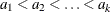 be a sequence of scores associated with the k samples. The test statistic and its standard error are given by
  and
and 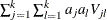 , respectively. Under , the z-score
![\[ Z = \frac{ \sum _{j=1}^ k a_ j v_ j}{\sqrt \{ \sum _{j=1}^ k \sum _{l=1}^ k a_ j a_ l V_{jl}\} } \]](images/statug_lifetest0286.png)
has, asymptotically, a standard normal distribution. PROC LIFETEST provides both one-tail and two-tail p-values for the test.