The LIFETEST Procedure

Breslow, Fleming-Harrington, and Kaplan-Meier Methods
Let  represent the distinct event times. For each
  , let
, let  be the number of surviving units (the size of the risk set) just prior to
  and let
  be the number of units that fail at . If the NOTRUNCATE option is specified in the FREQ statement, and can be nonintegers.
The Breslow estimate of the survivor function is
![\[ \hat{S}(t_ i) = \exp \biggl (-\sum _{j=1}^ i \frac{d_ j}{Y_ j} \biggr ) \]](images/statug_lifetest0045.png)
Note that the Breslow estimate is the exponentiation of the negative Nelson-Aalen estimate of the cumulative hazard function.
The Fleming-Harrington estimate (Fleming and Harrington 1984) of the survivor function is
![\[ \hat{S}(t_ i) = \exp \biggl (-\sum _{k=1}^ i\sum _{j=0}^{d_ k-1} \frac{1}{Y_ k-j} \biggr ) \]](images/statug_lifetest0046.png)
If the frequency values are not integers, the Fleming-Harrington estimate cannot be computed.
The Kaplan-Meier (product-limit) estimate of the survivor function at is the cumulative product
![\[ \hat{S}(t_ i) = \prod _{j=1}^ i \left( 1 - \frac{d_ j}{Y_ j} \right) \]](images/statug_lifetest0047.png)
Notice that all the estimators are defined to be right continuous; that is, the events at are included in the estimate of  . The corresponding estimate of the standard error is computed using Greenwood’s formula (Kalbfleisch and Prentice 1980) as
![\[ \hat{\sigma } \left( \hat{S}(t_ i) \right) = \hat{S}(t_ i) \sqrt { \sum _{j=1}^ i \frac{d_ j}{Y_ j(Y_ j-d_ j)} } ~ \]](images/statug_lifetest0049.png)
The first quartile (or the 25th percentile) of the survival time is the time beyond which 75% of the subjects in the population under study are expected to survive. It is estimated by
![\[ q_{.25} = \mr{min}\{ t_ j | \hat{S}(t_ j) < 0.75\} \]](images/statug_lifetest0050.png)
If  is exactly equal to 0.75 from
  to
to  , the first quartile is taken to be
  . If it happens that is greater than 0.75 for all values of t, the first quartile cannot be estimated and is represented by a missing value in
the printed output.
. If it happens that is greater than 0.75 for all values of t, the first quartile cannot be estimated and is represented by a missing value in
the printed output.
The general formula for estimating the 100pth percentile point is
![\[ q_{p} = \mr{min}\{ t_ j | \hat{S}(t_ j) < 1-p\} \]](images/statug_lifetest0055.png)
The second quartile (the median) and the third quartile of survival times correspond to p = 0.5 and p = 0.75, respectively.
Brookmeyer and Crowley (1982) have constructed the confidence interval for the median survival time based on the confidence interval for the  . The methodology is generalized to construct the confidence interval for the 100pth percentile based on a g-transformed confidence interval for (Klein and Moeschberger 1997). You can use the CONFTYPE= option to specify the g-transformation. The
  % confidence interval for the first quantile survival time is the set of all points t that satisfy
![\[ \biggl | \frac{ g(\hat{S}(t)) - g(1 - 0.25)}{g'(\hat{S}(t)) \hat{\sigma }(\hat{S}(t))} \biggr | \leq z_{1-\frac{\alpha }{2}} \]](images/statug_lifetest0056.png)
where  is the first derivative of
  and
and  is the
  th percentile of the standard normal distribution.
Consider the bone marrow transplant data described in Example 70.2. The following table illustrates the construction of the confidence limits for the first quartile in the ALL group. Values
of  that lie between
  =
=  1.965 are highlighted.
|
Constructing 95% Confidence Limits for the 25th Percentile |
|||||||
|---|---|---|---|---|---|---|---|
|
|
|||||||
|
t |
|
|
LINEAR |
LOGLOG |
LOG |
ASINSQRT |
LOGIT |
|
1 |
0.97368 |
0.025967 |
8.6141 |
2.37831 |
9.7871 |
4.44648 |
2.47903 |
|
55 |
0.94737 |
0.036224 |
5.4486 |
2.36375 |
6.1098 |
3.60151 |
2.46635 |
|
74 |
0.92105 |
0.043744 |
3.9103 |
2.16833 |
4.3257 |
2.94398 |
2.25757 |
|
86 |
0.89474 |
0.049784 |
2.9073 |
1.89961 |
3.1713 |
2.38164 |
1.97023 |
|
104 |
0.86842 |
0.054836 |
2.1595 |
1.59196 |
2.3217 |
1.87884 |
1.64297 |
|
107 |
0.84211 |
0.059153 |
1.5571 |
1.26050 |
1.6490 |
1.41733 |
1.29331 |
|
109 |
0.81579 |
0.062886 |
1.0462 |
0.91307 |
1.0908 |
0.98624 |
0.93069 |
|
110 |
0.78947 |
0.066135 |
0.5969 |
0.55415 |
0.6123 |
0.57846 |
0.56079 |
|
122 |
0.73684 |
0.071434 |
–0.1842 |
–0.18808 |
–0.1826 |
–0.18573 |
–0.18728 |
|
129 |
0.71053 |
0.073570 |
–0.5365 |
–0.56842 |
–0.5222 |
–0.54859 |
–0.56101 |
|
172 |
0.68421 |
0.075405 |
–0.8725 |
–0.95372 |
–0.8330 |
–0.90178 |
–0.93247 |
|
192 |
0.65789 |
0.076960 |
–1.1968 |
–1.34341 |
–1.1201 |
–1.24712 |
–1.30048 |
|
194 |
0.63158 |
0.078252 |
–1.5133 |
–1.73709 |
–1.3870 |
–1.58613 |
–1.66406 |
|
230 |
0.60412 |
0.079522 |
–1.8345 |
–2.14672 |
–1.6432 |
–1.92995 |
–2.03291 |
|
276 |
0.57666 |
0.080509 |
–2.1531 |
–2.55898 |
–1.8825 |
–2.26871 |
–2.39408 |
|
332 |
0.54920 |
0.081223 |
–2.4722 |
–2.97389 |
–2.1070 |
–2.60380 |
–2.74691 |
|
383 |
0.52174 |
0.081672 |
–2.7948 |
–3.39146 |
–2.3183 |
–2.93646 |
–3.09068 |
|
418 |
0.49428 |
0.081860 |
–3.1239 |
–3.81166 |
–2.5177 |
–3.26782 |
–3.42460 |
|
466 |
0.46682 |
0.081788 |
–3.4624 |
–4.23445 |
–2.7062 |
–3.59898 |
–3.74781 |
|
487 |
0.43936 |
0.081457 |
–3.8136 |
–4.65971 |
–2.8844 |
–3.93103 |
–4.05931 |
|
526 |
0.41190 |
0.080862 |
–4.1812 |
–5.08726 |
–3.0527 |
–4.26507 |
–4.35795 |
|
609 |
0.38248 |
0.080260 |
–4.5791 |
–5.52446 |
–3.2091 |
–4.60719 |
–4.64271 |
|
662 |
0.35306 |
0.079296 |
–5.0059 |
–5.96222 |
–3.3546 |
–4.95358 |
–4.90900 |


Consider the LINEAR transformation where  . The event times that satisfy
 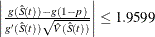 include 107, 109, 110, 122, 129, 172, 192, 194, and 230. The confidence of the interval [107, 230] is less than 95%. Brookmeyer
and Crowley (1982) suggest extending the confidence interval to but not including the next event time. As such the 95% confidence interval
for the first quartile based on the linear transform is [107, 276). The following table lists the confidence intervals for
the various transforms.
include 107, 109, 110, 122, 129, 172, 192, 194, and 230. The confidence of the interval [107, 230] is less than 95%. Brookmeyer
and Crowley (1982) suggest extending the confidence interval to but not including the next event time. As such the 95% confidence interval
for the first quartile based on the linear transform is [107, 276). The following table lists the confidence intervals for
the various transforms.
|
95% CI’s for the 25th Percentile |
||
|---|---|---|
|
CONFTYPE |
[Lower |
Upper) |
|
LINEAR |
107 |
276 |
|
LOGLOG |
86 |
230 |
|
LOG |
107 |
332 |
|
ASINSQRT |
104 |
276 |
|
LOGIT |
104 |
230 |
Sometimes, the confidence limits for the quartiles cannot be estimated. For convenience of explanation, consider the linear
transform . If the curve that represents the upper confidence limits for the survivor function lies above 0.75, the upper confidence
limit for first quartile cannot be estimated. On the other hand, if the curve that represents the lower confidence limits
for the survivor function lies above 0.75, the lower confidence limit for the quartile cannot be estimated.
The estimated mean survival time is
![\[ \hat{\mu } = \sum _{i=1}^ D \hat{S}(t_{i-1})(t_ i - t_{i-1}) \]](images/statug_lifetest0068.png)
where  is defined to be zero. When the largest observed time is censored, this sum underestimates the mean. The standard error of
 is estimated as
![\[ \hat{\sigma }(\hat{\mu }) = \sqrt {\frac{m}{m-1} \sum _{i=1}^{D-1} \frac{d_ i A_ i^2}{Y_ i (Y_ i - d_ i)} } \]](images/statug_lifetest0071.png)
where
![\begin{eqnarray*} A_ i & = & \sum _{j=i}^{D-1} \hat{S}(t_ j)(t_{j+1} - t_ j) \\[0.05in] m & = & \sum _{j=1}^ D d_ j ~ \\ \end{eqnarray*}](images/statug_lifetest0072.png)
If the largest observed time is not an event, you can use the TIMELIM= option to specify a time limit L and estimate the mean survival time limited to the time L and its standard error by replacing k by k + 1 with  .
.
Nelson-Aalen Estimate of the Cumulative Hazard Function
The Nelson-Aalen cumulative hazard estimator, defined up to the largest observed time on study, is
![\[ \tilde{H}(t) = \sum _{t_ i\leq t} \frac{d_ i}{Y_ i} \]](images/statug_lifetest0074.png)
and its estimated variance is
![\[ \hat{\sigma }^2 \left( \tilde{H}(t) \right) = \sum _{t_ i\leq t} \frac{d_ i}{Y_ i^2} \]](images/statug_lifetest0075.png)
Adjusted Kaplan-Meier Estimate
PROC LIFETEST computes the adjusted Kaplan-Meier estimate (AKME) of the survivor function if you specify both METHOD=KM and
the WEIGHT statement. Let ( denote an independent sample of right-censored survival data, where
  is the possibly right-censored time,
  is the censoring indicator (
 if is censored and
  if is an event time), and
  is the weight (from the WEIGHT statement). Let
  be the D distinct event times in the sample. At time
  , there are
  events out of
  subjects. The weighted number of events and the weighted number at risk are
  and
and  , respectively. The AKME (Xie and Liu 2005) is
![\[ \hat{S}(t) = \left\{ \begin{array}{ll} 1 & \mbox{if } t<t_1 \\ \prod _{t_ j \leq t} \left[ 1- \frac{d^ w_{j}}{Y^ w_{j}}\right] & \mbox{if } t \geq t_1 \end{array} \right. \]](images/statug_lifetest0088.png)
The estimated variance of is
![\[ \hat{\sigma }^2\left(\hat{S}(t) \right) = \left(\hat{S}(t)\right)^2 \sum _{j:t_ j \leq t} \frac{d^ w_{j}/Y^ w_{j}}{M_{j} (1-d^ w_{j}/Y^ w_{j})} \]](images/statug_lifetest0089.png)
where
![\[ M_{j} = \frac{\left(\sum _{i:T_ i \geq t_ j} w_ i \right)^2}{ \sum _{i:T_ i \geq t_ j} w_ i^2} \]](images/statug_lifetest0090.png)