The LIFEREG Procedure
- Overview
-
Getting Started

-
Syntax
-
DetailsMissing ValuesModel SpecificationComputational MethodSupported DistributionsPredicted ValuesConfidence IntervalsFit StatisticsProbability PlottingINEST= Data SetOUTEST= Data SetXDATA= Data SetComputational ResourcesBayesian AnalysisDisplayed Output for Classical AnalysisDisplayed Output for Bayesian AnalysisODS Table NamesODS Graphics
-
ExamplesMotorette FailureComputing Predicted Values for a Tobit ModelOvercoming Convergence Problems by Specifying Initial ValuesAnalysis of Arbitrarily Censored Data with Interaction EffectsProbability Plotting—Right CensoringProbability Plotting—Arbitrary CensoringBayesian Analysis of Clinical Trial DataModel Postfitting Analysis
- References
Example 69.8 Model Postfitting Analysis
PROC LIFEREG enables you to make model-based inferences. This example uses the larynx cancer data (Klein and Moeschberger 1997) to illustrate usage of the LSMEANS, LSMESTIMATE, and EFFECTPLOT statements for model postfitting analysis.
The survival time is modeled by a proportional odds model with two covariates: patient age and cancer stage (1, 2, 3, 4). The following statements use PROC LIFEREG to fit this model:
ods graphics on;

proc sort data=Larynx;
   by DESCENDING Stage;
run;

proc lifereg data=Larynx order=data;
   class Stage;
   model Time*Death(0) = Age Stage / dist = llogistic;
   lsmeans Stage / diff adjust=Sidak;
   effectplot / noobs;
run;
The LSMEANS statement compares pairwise differences in survival times among the four different cancer stages, while adjusting for age. The ADJUST=SIDAK option uses the Sidak method to control the overall Type I error rate of these comparisons. Results are displayed in Output 69.8.1.
Output 69.8.1: LS-Means Differences between Disease Stages
| Differences of Stage Least Squares Means Adjustment for Multiple Comparisons: Sidak |
||||||
|---|---|---|---|---|---|---|
| Stage | _Stage | Estimate | Standard Error | z Value | Pr > |z| | Adj P |
| 4 | 3 | -0.9604 | 0.4379 | -2.19 | 0.0283 | 0.1581 |
| 4 | 2 | -1.6404 | 0.4931 | -3.33 | 0.0009 | 0.0053 |
| 4 | 1 | -1.7661 | 0.4257 | -4.15 | <.0001 | 0.0002 |
| 3 | 2 | -0.6800 | 0.4316 | -1.58 | 0.1151 | 0.5199 |
| 3 | 1 | -0.8057 | 0.3539 | -2.28 | 0.0228 | 0.1292 |
| 2 | 1 | -0.1257 | 0.4152 | -0.30 | 0.7621 | 0.9998 |
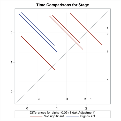
All the LS-means differences and their significance are displayed by the mean-mean scatter plot in Output 69.8.2.
Output 69.8.2: Plot of Pairwise LS-Means Differences
Suppose you want to jointly test whether the effects of stages 2, 3, and 4 are different from stage 1. The following LSMESTIMATE statement contrasts the LS-means of stages 2, 3, and 4 against the LS-means of stage 1:
proc lifereg data=Larynx order=data;
   class Stage year;
   model Time*Death(0) = Age Stage / dist = llogistic;
   lsmestimate Stage 'Stage 4 vs 1' 1 0 0 -1,
                     'Stage 3 vs 1' 0 1 0 -1,
                     'Stage 2 vs 1' 0 0 1 -1 / cl adjust=Sidak;
run;
The CL option produces 95% confidence limits, including both unadjusted ones and those adjusted for multiple comparisons according to the ADJUST= option. Results are displayed in Output 69.8.3.
Output 69.8.3: Custom LS-Means Tests and Relative Odds
| Least Squares Means Estimates Adjustment for Multiplicity: Sidak |
|||||||||||
|---|---|---|---|---|---|---|---|---|---|---|---|
| Effect | Label | Estimate | Standard Error | z Value | Pr > |z| | Adj P | Alpha | Lower | Upper | Adj Lower | Adj Upper |
| Stage | Stage 4 vs 1 | -1.7661 | 0.4257 | -4.15 | <.0001 | 0.0001 | 0.05 | -2.6004 | -0.9319 | -2.7825 | -0.7498 |
| Stage | Stage 3 vs 1 | -0.8057 | 0.3539 | -2.28 | 0.0228 | 0.0668 | 0.05 | -1.4993 | -0.1122 | -1.6507 | 0.03921 |
| Stage | Stage 2 vs 1 | -0.1257 | 0.4152 | -0.30 | 0.7621 | 0.9865 | 0.05 | -0.9395 | 0.6881 | -1.1171 | 0.8657 |
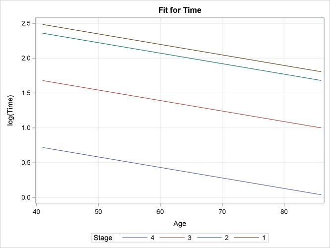
As displayed in Output 69.8.4, the EFFECTPLOT statement generates a plot of age effects on survival time on a natural logarithm scale by four disease stages.
Output 69.8.4: Age Effects by Disease Stages
You can also perform the preceding analysis for a Bayesian model. The following statements generate posterior samples from a Bayesian model and request an LS-means analysis to compare the stage effects:
proc lifereg data=Larynx order=data;
   class Stage;
   model Time*Death(0) = Age Stage / dist = llogistic;
   bayes seed=100 nmc=500 nbi=500 diagnostic=none outpost=OOO;
   lsmeans Stage / diff exp;
   lsmestimate Stage 'Stage 4 vs 1' 1 0 0 -1,
                     'Stage 3 vs 1' 0 1 0 -1,
                     'Stage 2 vs 1' 0 0 1 -1
                        / cl plots=boxplot(orient=horizontal);
run;
Because no prior distributions for the regression coefficients were specified, the default uniform improper distributions shown in the "Uniform Prior for Regression Coefficients" table in Output 69.8.5 are used. The specified gamma prior for the scale parameter is also shown in Output 69.8.5.
Output 69.8.5: Model Parameter Priors
Under the Bayesian framework, the LS-means differences are treated as random variables for which posterior samples are readily available according to the linear relationship of LS-means and the regression coefficients. Output 69.8.6 lists the sample mean, standard deviation, and percentiles for each LS-means difference.
Output 69.8.6: LS-Means Differences between Disease Stages
| Sample Differences of Stage Least Squares Means | ||||||||||||
|---|---|---|---|---|---|---|---|---|---|---|---|---|
| Stage | _Stage | N | Estimate | Standard Deviation | Percentiles | Exponentiated | Standard Error of Exponentiated |
Percentiles for Exponentiated |
||||
| 25th | 50th | 75th | 25th | 50th | 75th | |||||||
| 4 | 3 | 500 | -0.9307 | 0.4752 | -1.2743 | -0.9446 | -0.6086 | 0.4426 | 0.232690 | 0.2796 | 0.3888 | 0.5441 |
| 4 | 2 | 500 | -1.6591 | 0.5327 | -2.0161 | -1.6573 | -1.2861 | 0.2181 | 0.115808 | 0.1332 | 0.1907 | 0.2763 |
| 4 | 1 | 500 | -1.8001 | 0.4321 | -2.0951 | -1.7943 | -1.5491 | 0.1815 | 0.082975 | 0.1231 | 0.1663 | 0.2124 |
| 3 | 2 | 500 | -0.7284 | 0.4828 | -1.0488 | -0.7219 | -0.3975 | 0.5410 | 0.268735 | 0.3504 | 0.4858 | 0.6720 |
| 3 | 1 | 500 | -0.8694 | 0.3727 | -1.1199 | -0.8541 | -0.6149 | 0.4488 | 0.168055 | 0.3263 | 0.4257 | 0.5407 |
| 2 | 1 | 500 | -0.1410 | 0.4413 | -0.4126 | -0.1417 | 0.1363 | 0.9585 | 0.462376 | 0.6619 | 0.8679 | 1.1461 |
The LSMESTIMATE statement produces summary statistics of the posterior samples for the specified LS-means contrasts. Results are presented in Output 69.8.7; they are very similar to the results based on maximum likelihood in Output 69.8.3.
Output 69.8.7: Summary Statistics of Custom LS-Means Differences
| Sample Least Squares Means Estimates | ||||||||||
|---|---|---|---|---|---|---|---|---|---|---|
| Effect | Label | N | Estimate | Standard Deviation | Percentiles | Alpha | Lower HPD | Upper HPD | ||
| 25th | 50th | 75th | ||||||||
| Stage | Stage 4 vs 1 | 500 | -1.8001 | 0.4321 | -2.0951 | -1.7943 | -1.5491 | 0.05 | -2.6279 | -0.8897 |
| Stage | Stage 3 vs 1 | 500 | -0.8694 | 0.3727 | -1.1199 | -0.8541 | -0.6149 | 0.05 | -1.6033 | -0.2031 |
| Stage | Stage 2 vs 1 | 500 | -0.1410 | 0.4413 | -0.4126 | -0.1417 | 0.1363 | 0.05 | -1.1401 | 0.6252 |
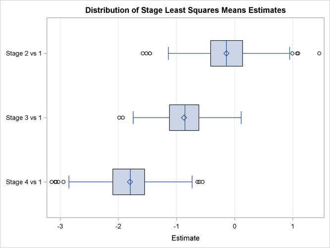
The PLOTS= option uses ODS Graphics to display the Bayesian samples. A box plot is presented in Output 69.8.8.
Output 69.8.8: Box Plot of Sampled LS-Means Differences